What is homeostasis? All biological systems have evolved mechanisms that allow them to keep functioning despite large changes in their inputs, their environments, and, indeed, large changes in their own component par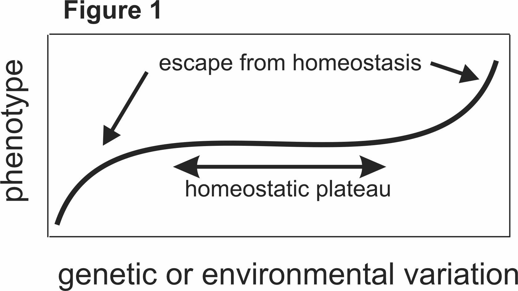 ts. We call this general concept “homeostasis,’’ some would call it robustness, and, as we will see below, homeostasis is created by evolved control mechanisms within the biological systems themselves. Conceptually, one can recognize homeostasis when a phenotype depends on genetic or environmental variation through a chair shaped curve as in Figure 1. Over a large middle region of variation, the phenotype hardly changes at all because of control mechanisms, but when the variation becomes too large one loses the phenotype, a phenomenon that we call “escape from homeostasis [1],” because the control mechanisms are no longer effective. We will see lots of specific examples below.
Such homeostatic mechanisms occur at all spatial scales, from gene regulatory networks to cell biochemistry to whole organ or whole-body physiology to ecosystems. And mechanisms at one scale can affect or create homeostasis at other scales. For example, metabolites can bind to gene promoter regions affecting gene expression, and metabolites in cells are the building blocks of whole organ and whole-body physiology.
Typically, homeostasis is an observed property, and it is the job of biologists and mathematicians to understand the mechanisms that create it. On a fundamental level, one cannot understand how a biological system works without understanding the homeostatic control mechanisms. And, as we shall see, understanding when homeostatic mechanisms work and don’t work is important for disease progression, treatment, and drug design. Finally, the study of homeostatic mechanisms is important for understanding evolution, because evolution selects phenotypes and cannot select amongst the underlying variation if the phenotypes are the same.
Classical Physiological homeostasis. The concept of homeostasis has a long history in physiology going back to the French physiologist Claude Bernard who emphasized the importance of maintaining “le milieu intérieur”. The word homeostasis itself was introduced in 1926 by the American physiologist Walter Bradford Cannon (reference in [2]). In studying homeostasis, classical physiologists were mainly concerned with the mechanisms t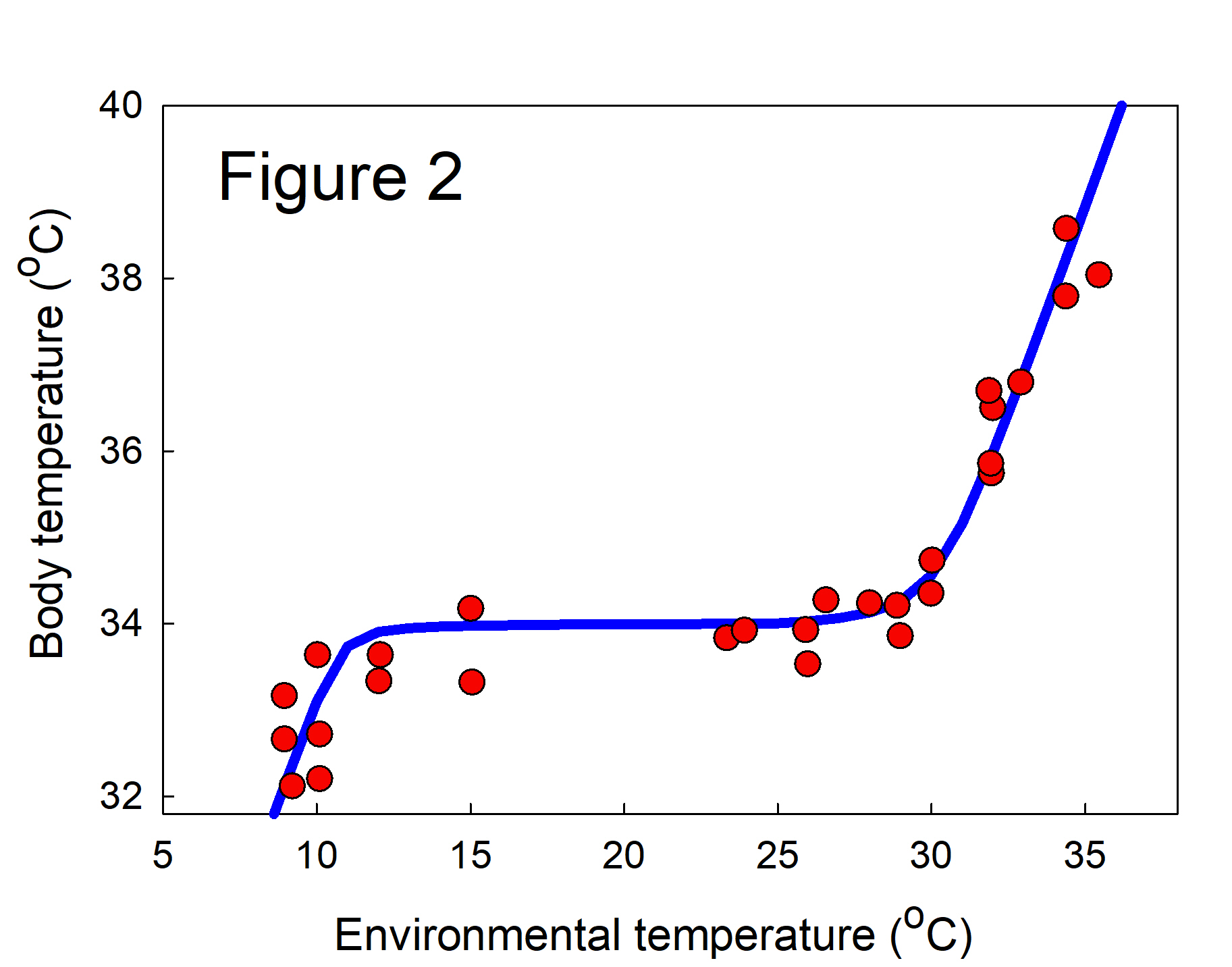 hat regulated whole body variables like temperature, plasma sodium and glucose levels, and muscle tone, and kept them within certain narrow limits. In Figure 2, the phenotypic variable is body temperature and the environmental variable is ambient temperature. The data points are measurements of body temperature in the brown opossum [1] and we have drawn the chair curve through the data. The mechanisms of body temperature regulation are well known. One can clearly see the homeostatic plateau and the upper and lower temperatures where the mechanisms can no longer compensate for the ambient temperature.
Figure 3 shows another example of classical physiological homeostasis. The phenotypic variable is cerebral blood flow in h umans and the environmental variable is cerebral blood pressure. Because of numerous homeostatic mechanisms, the cerebral blood flow shows remarkable homeostasis over a wide range of pressures. LLA and ULA indicate the lower and upper limits of pressures between which the mechanisms work well. Once one leaves the homeostatic region, serious health effects occur. MAP indicates the mean arterial pressure while resting. One can clearly see the chair curve and the escape from homeostasis. References can be found in [2].
Why is biochemistry so difficult and important? We are being provocative because many researchers (and medical students!) think that biochemistry is a very old-fashioned subject where all was known long ago and summarized on the famous chart of cell metabolism that hangs in high school biology classrooms. In this old-fashioned biochemistry one studies, often in test tube experiments, how an amino acid, A, is transformed by a sequence of enzymatic steps into the end-product P. But how does this pathway work in real cells where other pathways use the same amino acid, and where myriad allosteric control mechanisms utilizing other substrates affect the steps of the pathway? Further, the steps of the pathway are catalyzed by enzymes whose expression levels differ by cell type and differ in the same cell type between individuals, and the genes for enzymes have many polymorphisms that increase or decrease the activity of the enzymes. Even more daunting, cell metabolism must accommodate dramatic changes in amino acid input due to meals and many enzymes need vitamin co-factors, so diet plays an important role. Finally, many enzymes and the genes that code for them are affected by endocrine regulators, so one expects cell metabolism to be different in men and women [3].
Even in classical biochemistry, homeostatic mechanisms were understood to play an important role. Because of Michaelis-Menten kinetics (or fancier variants), the flux is almost constant when the substrate concentration is very high. It was understood that end-product inhibition [2], in which the end-product inhibits one or more enzymes in its synthetic pathway, is a control mechanism to prevent too much buildup of the product. And substrate inhibition, in which the substrate itself inhibits the enzyme, is a control mechanism that prevents too much flux from going down the pathway [4]. Here, we want to explain four more subtle mechanisms that show how cells can evolve homeostatic mechanisms solve difficult challenges in variable environments. These four examples will allow us to explain why the study of homeostatic mechanisms is crucial, both for medicine and for the theory of evolution.
The first three examples come from one carbon metabolism (OCM); a simplified schematic diagram is shown in Figure 4. The rectangular boxes represent substrates and the blue ovals contain the acronyms of the enzymes that catalyze the reactions. Full names of metabolites and enzymes can be found in Figure 1 of [3]. A few remarks are in order to explain why OCM is so well-studied and so important for human health. OCM is so named because one carbon groups are being transferred from one molecule to another. The amino acid methionine is the input to the four green metabolites of the methionine cycle. SAM is the universal methyl group donor in cells, which means that SAM is a substrate for reactions in which a methyl group from SAM is attached to some other substrate. For example, in the GNMT reaction the substrates glycine and SAM are converted to sarcosine and SAH. The substrates that receive the methyl group from SAM in the other four reactions are not shown. Arsenic is detoxified in the liver by the AS3MT reaction. Cytosines in DNA are methylated by the DNMT reaction; this is the basis of epigenetics. The GAMT reaction is the last step in creatine synthesis. The PEMT reaction is the first step in the pathway that synthesizes choline, which is important for cell membranes.
Homocysteine (Hcy) is the major biomarker for cardiovascular disease. The CBS reaction is the first step in the pathway that creates glutathione, the main antioxidant in the cell. In the folate cycle, the six metabolites are different forms of folate (vitamin B9). The AICART and TS reactions are crucial steps in the synthesis of purines and pyrimidines, respectively.
It is a mistake to regard OCM in Figure 4 as static. In fact, it is dynamic and changing all the time. After meals, the methionine input goes up by a factor of 2 to 6. If the cell is dividing once a day, the genes for the enzymes in the folate cycle are upregulated by a factor of 100 because the cell has to create approximately 35,000 new base pairs per second all day. We note that the enzyme MS requires vitamin B12 as a co-factor and the enzymes CBS and SHMT require vitamin B6 as a co-factor, so diet directly affects OCM. In addition, estrogen and testosterone affect the enzymes SHMT, MTHFR, MS, BHMT, CBS and PEMT and cause their expression levels to be quite different in men and women [3].
Example 1. Conservation of mass in the methionine cycle, stabilization of SAM. Since SAM is the universal methyl group donor in the cell (there are 150 methyl transferase reactions, not just the 5 depicted in Figure 4), it seems advantageous for the cell to stabilize the SAM concentration so it doesn’t change too much. Since the methionine input changes by a factor of 2-6 after meals, how is this accomplished? Note that if all the arrows in Figure 4 represented reactions that depend linearly on their substrates the concentration of SAM at steady state would depend linearly on the methionine input. The reactions are not linear, they are Michaelis-Menten (with modifications), but the question remains how SAM is stabilized. This is accomplished by two of the red arrows in Figure 4: SAM activates the enzyme CBS and SAM inhibits the enzyme BHMT. This means that as the methionine input goes up and SAM starts to rise, more of the mass arriving at Hcy from SAH is directed down the transsulfuration pathway and less mass flows from Hcy to Met (which is called remethylation). Conversely, when methionine input goes down (for example, overnight), and SAM starts to decrease, the activation of CBS is partially withdrawn as is the inhibition of BHMT, so less mass goes down the transsulfuration pathway and more mass is sent from Hcy to Met. These two allosteric interactions make the changes in SAM quite modest, despite large changes in methionine input due to meals. Using the mathematical model, one can quantify what one means by “modest” [5].
Example 2. Competing methyl transferases. The cell faces another difficult regulatory challenge. Each of the 150 methyl transferase reactions uses SAM as the substrate. The concentrations of the enzymes for each of these reactions are not constant but change as the cell upregulates or downregulates the corresponding genes. For example, if there is sufficient creatine in the diet, the concentration of GAMT is very low and the flux through that arrow is small. But if there is little creatine in the diet, the concentration of GAMT is high and the flux on the GAMT pathway is high. This presents the cell with a problem. If the flux through the GAMT pathway increases a lot then SAM concentration will go down, and this will affect all the other methyl transferase pathways. The cell solves this problem with the other two red arrows in Figure 4: SAM inhibits MTHFR (in the folate cycle) and its product, 5mTHF, inhibits the methyl transferase GNMT. Here’s how this works. Suppose that GAMT flux increases and SAM starts to go down. Then some of the inhibition of MTFR is withdrawn so the concentration of 5mTHF will rise inhibiting GNMT so the flux in the GNMT pathway goes down, which keeps the concentration of SAM up. Conversely, suppose that GAMT flux decreases and SAM starts to go up. Then the inhibition of MTFR is increased so the concentration of 5mTHF will fall removing inhibition of GNMT so the flux in the GNMT pathway goes up, which keeps the concentration of SAM down. This mechanism is investigated in [6].
Long-range interactions and the need for mathematics. We call the red arrows in Figure 4 “long-range interactions” because substrates influence distant enzymes in the network. Note that we assume the cell is well-mixed chemically, so we don’t mean spatially long-range in the cell, we mean long-range in the network. In the old biochemistry, one could use pathway diagrams to decide what will happen if one intervenes, say by adding a lot of one substrate. One just looks where that substrates is used and then guesses that the downstream concentrations in the pathways will rise. But, if there are long-range interactions where concentrations affect distant enzymes one can’t “see” what the effects will be. You need a mathematical model so that you can compute what the effects will be. In [2], we discuss 4 different homeostatic motifs for long-range interactions: feedback inhibition; feedforward excitation; parallel inhibition; and substrate inhibition. SAH inhibits all the methyl transferases so that’s an example of feedback inhibition. SAM activates CBS, so that is an example for feedforward activation. The effect of SAM on MTHFR and the effect of 5mTHF on GNMT is an example of the parallel inhibition motif. And substrate inhibition in the folate cycle is discussed next. So, all of these different regulatory motifs occur in this one diagram. And, there are other regulations that we haven’t mentioned! SAM excites MATI and inhibits MATIII and choline produces betaine that excites both BHMT and CBS. It’s good to remember that the folate and methionine cycles are very ancient (they occur in bacteria), so nature has had a lot of time to find and tune these regulatory mechanisms in order to create functional homeostasis.
Example 3. Folate homeostasis. Before talking about folate, we need to discuss substrate inhibition, a concept introduced by Haldane in 1930. Suppose that an enzyme has two receptors for a substrate, S, a catalytic site and an allosteric site. If only the catalytic site is bound the product, P, is produced at a rate k2 but if both are bound, P is produced at a much lower rate k4; see Figure 5. A simple case would be when k4 = 0. Then, as total substrate increases more and more of the enzyme is tied in the ternary complexes where two substrate molecules and bound to the enzyme, so the velocity of the reaction will go to zero as the concentration of S goes to infinity. Many biologically important enzymes show substrate inhibition [4], but substrate inhibition has been largely ignored by the chemistry, biology, and mathematical biology communities. We will explain how it plays a role in folate homeostasis.
There are six folate substrates in the folate cycle and all of them bind allosterically to one or more of the many enzymes in the cycle, not necessarily the enzyme that catalyzes the reaction for which they are the substrate. This is a kind of “group” substrate inhibition, in which many folate molecules can’t be substrates because they are bound allos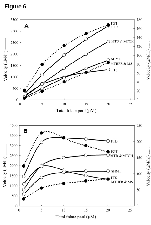 terically, and many enzymes molecules can’t catalyze reactions because they are bound allosterically. This seems quite weird and unproductive but it causes homeostasis of reactions velocities with respect to total liver folate. The normal total concentration of folate in human liver is about 20mM, but, of course, that varies depending on the diet of the individual. We get our folate by eating green vegetables. Figure 6, Panel A shows the reaction velocities of several of the reactions in the folate cycle as a function of total liver folate if substrate inhibition is not put in the mathematical model. Basically, all the reaction velocities go approximately linearly to zero as total folate decreases from 20mM to 0. However, if substrate inhibition is included in the model, then the reaction velocities stay near normal even when total folate declines from 20mM to 5mM; see Figure 6, Panel B. Figure 6 is taken from [7].
Here is the physiological significance. The half-life of folate in the body is about 3 months, so if you don’t eat any green vegetables for 3 months your folate with drop to 10mM. It does matter, because of the substrate inhibition, the velocities stay high. Now if you don’t eat any green vegetables for another 3 months your total folate would drop to 5mM, but that still doesn’t affect the velocities very much. What is the cause of this remarkable homeostasis? As total folate drops, the reversible reactions by which folate are allosterically bound to folate enzymes tend to dissociate, releasing free folate and free enzymes that can be used in the reactions. It is tempting to speculate that this substrate inhibition and folate homeostasis was a mechanism to get our ancestors through Winter when few vegetables would have been available.
Example 4. Dopamine homeostasis. Dopamine is a catecholamine that is used as a neurotransmitter both in the periphery and in the central nervous system. Dysfunction in various dopaminergic systems is known to be associated with various disorders, including schizophrenia, Parkinson’s disease, and Tourette’s syndrome. Furthermore, microdialysis studies have shown that addictive drugs increase extracellular dopamine and brain imaging has shown a correlation between euphoria and psychostimulant-induced increases in extracellular dopamine. These consequence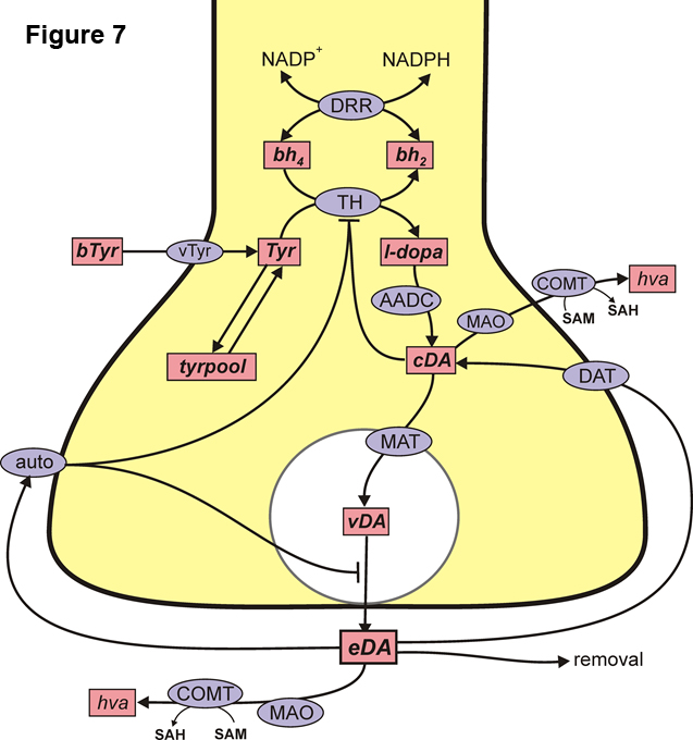 s of dopamine dysfunction indicate the importance of maintaining dopamine functionality through homeostatic mechanisms that create a stable balance between synthesis, storage, release, catabolism, and reuptake.
Figure 7 shows a schematic diagram of the main pathways involved in brain dopamine metabolism [8]. In dopamine neurons, dopamine (DA) is synthesized from the amino acid tyrosine which is imported from the blood. The enzyme tyrosine hydroxylase adds an -OH group and the enzyme AADC cuts off the carboxyl group to make cytosolic DA (cda). Cytosolic DA is rapidly packaged into vesicles (vda) and is released into the extracellular space (eda) when the action potential arrive at the synapse or varicosity. DA is catabolized in the cytosol by the enzyme MAO and some extracellular DA is transported into glial cells where it is catabolized by MAO. But most eda is transported back into the cytosol by the dopamine transporter DAT. The autoreceptors (auto) sense extracellular DA and when it is too high, they inhibit synthesis and release. When eda is too low, the autoreceptors remove some inhibition so synthesis and release are increased.
Thus, the auroreceptors are a homeostatic mechanism to keep extracellular DA within fairly narrow limits. Figure 8, taken from [1], shows how good this mechanism is. Both TH and D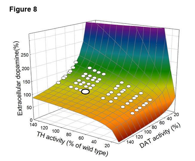 AT have common polymorphisms in the human population and these polymorphisms are functional in the sense that when they are present the activity of TH and/or DAT changes a lot. Figure 8 shows a surface where the z-axis shows extracellular DA concentration relative to wild type (100\%) and the x and y axes are the activities of TH and DAT (again wild type is 100\%). The large white dot shows the extracellular DA concentration when TH and DAT are wild type (100\%). The high blue cliff in the back is where one goes in the presence of cocaine because cocaine blocks the DATs. The orange cliff in the front is where one falls in various diseases like Parkinson’s caused by low DA. But amazingly, all the common polymorphisms in the human population correspond to points of the flat part of the surface where extracellular DA doesn’t vary very much. Presumably, that’s why they are still common in the human population. Even though the polymorphisms have large functional effects on TH and DAT, it doesn’t matter because of the homeostasis that is created by the autoreceptors. Instead of a chair curve, here we have a two-dimensional homeostatic surface in three dimensions.
Homeostasis and precision medicine. The idea of personalized (or precision) medicine is that there is great biological variation and therefore patient treatments should be designed based on the individual characteristics of patients. What characteristics? Well, certainly their genotype, but also their diet, their exercise patterns, the air they breathe, and so forth. These other variables are very hard to quantify, especially since one would want to know them over the patient’s lifetime. But determining a patient’s genotype is cheap and easy. So, researchers expect that we can determine treatments based on genotype alone. But as the surface in Figure 8 shows, the genotype may be very different, but the phenotype (the extracellular dopamine concentration) may remain the same because of regulatory biochemical mechanisms. Thus, it unlikely that personalized medicine treatment strategies based on genotype alone will work well.
The concept of homeostasis gives us a mechanistic explanation of the term predisposition to disease that is often used in medicine based solely on data showing a statistical correlation between a disease and a genotype. Consider the surface in Figure 8, where the phenotypic variable is the extracellular DA concentration and the genetic variables are the activity of TH and DAT. The genotypes with very low TH activity are at the edge of the DA cliff; they are on the flat, homeostatic part of the DA surface, but barely. This surface was computed using our deterministic model and allowing only variation in TH and DAT activity. But (as explained in detail under the tab “population models”) there is a tremendous amount of variation in gene expression levels between individuals. If one includes this variation in a population model of the DA system then some of individuals with this genotype fall off the edge of the homeostatic plateau and have very low DA (see Figure 5 in [9]). Interestingly, these low TH genotypes sometimes show a dystonia, involuntary muscle contractions that affect posture, brought about by low levels of extracellular DA that can be alleviated by levodopa (reference in [10]). Their placement at the edge of the cliff predisposes them to the dystonia, which can be brought on by changes in the other variables that affect the shape of the surface.
Homeostasis and development. One of the most remarkable features of animal and plant development is its irrevocable directionality and the appearance of being goal-oriented. Severe insults during development, such a removal of part of an embryo, or of a developing appendage, can redirect development to repair the lesion and regenerate the missing parts to near normality. Developmental biologists call this robustness, but it almost certainly involves homeostatic biochemical mechanisms such as we have discussed as well as other mechanisms. The ability to flexibly structure a body in early embryogenesis is called regulative development, and stands in contrast to mosaic development in which missing parts cannot be replaced. Later in development, the ability to reconstruct missing parts is generally referred to as regeneration. Many authors have commented on the fact that development gives the appearance of being self-organizing and self-correcting and have suggested mechanisms by which this could occur. The most common mechanism invoked for self-organizing pattern formation in development is Turing’s reaction-diffusion system. However, this cannot provide the complete explanation because, typically, in mathematical models of Turing systems, the patterns are extremely sensitive to parameters. Gradients of morphogens are found throughout development and are involved in establishing axes of differentiation in developing limbs, craniofacial features, digit differentiation, insect wing venation patterning, color pattern development, and many others processes by which cells and tissues become different from one another. Diffusion gradients not only supply positional information, but can also be used to scale patterns to fields that vary in size and thus may provide a robustness mechanism for development. The morphogenetic gradients, peaks and valleys that are set up during development control downstream pathways that stimulate local growth, cell death, cell specialization and tissue differentiation. What is still missing in most if not all cases, is an understanding of how the “endpoint” is determined. How does a tissue, organ, or appendage “know” it has arrived at its final size and shape? For further discussion and references, see [11]
Homeostasis and evolution. The existence of homeostatic mechanisms provides new mechanisms in the theory of evolution as well as new challenges. We touch on a few of the ideas here; fuller discussions can be found in [9] and [11].
Cryptic Genetic variation. Consider the dopamine surface in Figure 8. Both TH and DAT have common polymorphisms in the human population and these polymorphisms are functional in the sense that they have large effects on the activities of TH and DAT. But, because of a homeostatic mechanism (the autoreceptors) the polymorphisms have very little effect on the phenotypic variable, the extracellular concentration of dopamine. Thus, evolution cannot select among these polymorphisms because the phenotypes are the same. This is called cryptic genetic variation.
Environmental change. The environment in which a biological organism exists can change and sometimes change rapidly. For humans, the climate changes, the types of food that are available may change, and novel human enemies or pathogens may appear. Such environmental change can affect a flat homeostatic surface and cause it to be tipped. Figure 9 shows an example from one carbon metabolisms. In Panel A, the phenotypic variable is the rate of the thymidylate synthase (TS) reaction which is a major step in making pyr imidines (see Figure 4). The surface shows the TS rate as a function of methylene tetrahydrofolate (MTHFR) activity and methionine synthase (MS) activity. The large white dot is the normal steady state in the model, which is in the middle of a homeostatic plateau. The smaller white dots are combinations of common polymorphisms in MTHFR and MS. As was the case with Figure 7, the polymorphisms are on the flat homeostatic part of the surface and so represent cryptic genetic variation. The enzyme MS requires vitamin B12 as a co-factor. Panel B shows what the surface looks like in the presence of a vitamin B12 deficiency. It is now steeply tipped so the different polymorphisms have a big effect on TS rate. Thus, selection can now operate on these polymorphisms because the phenotypes are different.
Rapid Evolution. As mutations accumulate in cryptic genetic variation presumably some of them are advantageous and some of then are deleterious. They are already present even though they are on the homeostatic surface and therefore have little effect. This means that when environmental change comes (as in Panel B), selection can act quickly to change the genome because the genetic variations are already present and ready to be selected on.
The diversity of the human genome. In the long history of the human species, until very recently local population groups were isolated from distant populations. And, the environmental changes, weather, food supply, existence of particular pathogens, were often local events. Thus, the rapid action of selection on cryptic genetic variation that has become uncryptic because of an environmental change, could act locally on small and medium sized populations. This is probably part of the reason for the diversity in the human genome.
References
[1] (2014) Escape from homeostasis. Nijhout HF, Best J, Reed, MC. Mathematical Biosciences 257, 104-110.
[2] (2017) Analysis of Homeostatic Mechanisms in Biochemical Networks. M. Reed, J. Best, M. Golubitsky, I. Stewart, H. F. Nijhout. Bulletin of Mathematical Biology, 79:2534-2557.
[3] (2018) Sex differences in hepatic one-carbon metabolism. F. Sadre-Marandi, T. Dahdoul, M. C. Reed, H. F. Nijhout. BMC Systems Biology, 12:89.
[4] (2010) The biological significance of substrate inhibition: A mechanism with many functions. Reed MC, Lieb, A., Nijhout HF. BioEssays 32, 422-429.
[5] (2006) Long-Range Allosteric Interactions between the Folate and Methionine Cycles Stabilize DNA Methylation Reaction Rate; Nijhout HF, Reed MC, Anderson DF, Mattingly JC, James SJ, Ulrich CM, Epigenetics, 1, 81-87.
[6] (2015) Mathematical analysis of the regulation of competing methyltransferases. Reed MC, Gamble MV, Hall MN Nijhout HF. BMC Systems Biology 9:69.
[7] (2004) A mathematical model of the folate cycle: New insights into folate homeostasis; Nijhout HF, Reed MC, Budu P, Ulrich CM, Journal of Biological Chemistry, 279, 55008-55016.
[8] (2009) Homeostatic mechanisms in dopamine synthesis and release: a mathematical model. Best J, Nijhout HF, Reed MC, Theoretical Biology and Medical Modelling 6, 21.
[9] (2017) Systems Biology of Phenotypic Robustness and Plasticity. H. F. Nijhout, F. Sadre-Marandi, J. Best, M. Reed. Integrative and Comparative Biology, 57: 171-184
[10] (2015) Using mathematical models to understand metabolism, genes and disease. Nijhout HF, Best JA, Reed MC. BMC Biology 13:79.
[11] (2018) Systems biology of robustness and homeostatic mechanisms. H. F. Nijhout, J. A. Best, M. C. Reed, WIREs Syst. Biol. Med. 2018;e1440.
[12] (2014) Homeostasis and dynamic stability of the phenotype link robustness and stability. Nijhout HF, Reed, MC. Integrative and Comparative Biology 54 , 264-275.
[13] (2017) Systems Biology of Phenotypic Robustness and Plasticity. H. F. Nijhout, F. Sadre-Marandi, J. Best, M. Reed. Integrative and Comparative Biology, 57: 171-184.
[14] (2018) Homeostasis despite instability. W. Duncan, J. Best, M. Golubitsky, H. F. Nijhout, M. Reed. Mathematical Biosciences, 300:130-137.