*This discussion follows part of the expository article “Systems Biology of robustness and homeostatic mechanisms” (2018, see publications). Full citations for references can be found there.
No two individuals are alike in genetic makeup, gene expression levels, or environmental exposures. Yet this variation is usually ignored, and measures of biological variables are given as means with standard deviations, where the mean represents the value for some idealized or “average” individual. Traditionally, medicine treats this average individual, but it is the goal of precision medicine to treat each person by taking in account his or her individual characteristics. For several reasons, this is a daunting task. Of course, an individual’s genome is easy to obtain, but gene expression levels vary by 25% from individual to individual (Oleksiak et al., 2002; Sigal et al., 2006), and the methylation patterns on the genes depends on life history. Furthermore, it is difficult to even imagine accurate and useful ways of quantifying life history of environmental input, including diet and exercise.
Biological variation poses analogous issues for those of us who make mathematical models of biological systems in order to understand how the systems work. For simplicity, we’ll consider a system of ordinary differential equations (ODEs) that models a biochemical network, although the ideas and methods can be used for gene regulatory networks, gene-metabolic systems, physiological, and developmental systems. In the model, one must choose Km and Vmax values for each enzyme, and constants that represent the strengths of allosteric interactions or rates of transport between compartments. Such “constants” have a wide range of values in the literature (often over two orders of magnitude) reflecting the varied circumstances in which they were measured. So, for each constant one chooses an average or representative value. One then has a mathematical model for an “average” or idealized biochemical network and one can perform in silico experiments with the model, compare the results to extant data, and investigate mechanism. But this avoids dealing with the enormous biological variation between individuals.
We address both the biological issues and the mathematical issues by making system population models of biological systems. This type of model was introduced in Duncan, Reed, & Nijhout (2013) and Nijhout & Paulsen (1997), and 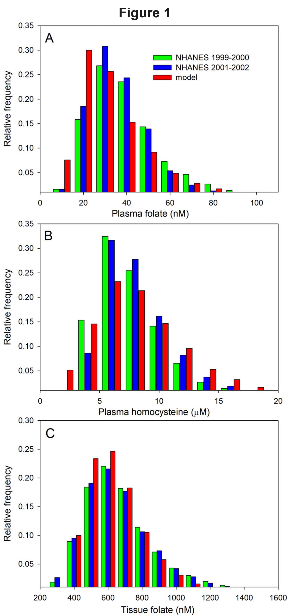 was reviewed in the mathematics literature by Swigon (2012). For a deterministic ODE model of a metabolic or physiological system, a system population model is constructed as follows. Each parameter has “normal value.” A new value for that parameter is selected from a probability distribution whose mean is the normal value. This is done independently for all (or a subset of) the parameters. The model is then run to equilibrium and the parameter values, metabolite concentrations, and fluxes are recorded. That is one virtual individual. This procedure is repeated 10,000 times to produce a database of 10,000 virtual individuals, each with different parameters, concentrations, and fluxes. But in each individual, the concentrations and fluxes depend on the chosen parameters through the same mechanism (the ODEs). Below, we briefly discuss how population models have been used.
Traditional statistical analysis. Since one has a large database of virtual individuals, one can utilize traditional statistical analyses to find new correlations, analyze scatterplots, and find individual outliers. The difference is that since the data all come from the same mechanistic model, one can conduct in silico experiments to understand the mechanisms that produce the correlations. We used this in Duncan et al. (2013a) and Duncan, Reed, and Nijhout (2013b) to show that plasma homocysteine is controlled by non-liver tissues, not by the liver. Of course, one should compare one’s virtual database to extant databases to verify that the model is good. The mathematical model of one carbon metabolism in the above papers produces population distributions of plasma folate, plasma homocysteine, and tissue folate given by the red bars in Figure 1 where one can compare the model distributions to the distributions in human populations obtained from the NHANES database (blue and green bars in Figure 1). One can see that our model produces a population distribution of these variables with an excellent fit to human population data. So, population models give another way to compare deterministic models to clinical data. In addition, Bayesian analysis of virtual population data, informed by a deterministic model, can also be used to identify candidate genes for particular traits or specific deviations from the wild type (Thomas et al., 2009).
Predisposition to disease. What does it mean to say that a genotype (or a life-style) “predisposes’’ you to a disease? Well, most simply, it means that there is a correlation between the genotype and the disease. But if a gene doesn’t cause the disease, what is the mechanism that gives this correlation, that predisposes one? We can use population m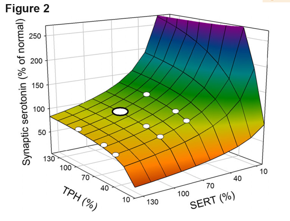 odels to give an explanation. We’ll consider a deterministic mathematical model of serotonin synthesis, storage in vesicles, release, and reuptake (Best et al. 2010a). Tryptophan hydroxylase (TPH) is the key enzyme for the synthesis of serotonin and the serotonin transporter (SERT) puts serotonin released into the extracellular space back into the cytosol. TPH and SERT have polymorphisms that are common in the human population that increase or decrease the efficacy of TPH and SERT. We used the mathematical model to compute extracellular serotonin as a function of the relative efficacy of TPH and SERT (with 100% being normal). The surface is shown in Figure 2. The large white dot is the “normal” steady value of extracellular serotonin and the small white dots show the value for various combinations of the common polymorphisms. Notice that all the polymorphisms are on the relatively flat part of the surface. Thos homeostasis is caused by the serotonin autoreceptors. These calculations are for the “average” individual, that is they were done with the deterministic model. Notice, however, that several polymorphism combinations are close to the edge of the cliff where serotonin drops rapidly. Individuals with those polymorphisms are predisposed to low serotonin, because if one varies all the parameters as we do in a population model the shape of the homeostatic plateau will change, and for some individuals, these polymorphisms may fall off the plateau. Such individuals will have very low serotonin. An analysis of the virtual population may identify the particular combinations of parameter values that make individuals more or less susceptible to develop low serotonin. An example of such a study, for individual variation of dopamine levels, is shown in Figure 5 of Nijhout et al. (2017).
Relating deterministic models to biological data. Imagine an experiment where a experimenter changes the input to a biochemical network for a short period of time and then measures the values of a particular concentration over time. If the experiment is repeated several times, somewhat different curves will be obtained, and the experimenter will report the mean curve and the standard deviations. In a system population model, each different choice of parameters (individuals) will produce a different curve. It is this family of model output curves that should be compared to the family of experimental curves, not just the average model curve to the experimental mean curve, because there is real biological information in the dispersion of the curves. Thus, system population models are the right way to compare mechanistic ODE models to real biological data. Figure 3 gives an example taken from our recent paper, “Autoreceptor control of serotonin dynamics.” The medial forebrain bundle of mice was stimulated and the antidromic spikes stimulate the dorsal raphe nucleus that send serotonin projections all over the brain. Extracellular serotonin was measure over 30 seconds in the hippocampus and Figure 3(a) shows the resulting family of response curve for 17 mice. The dark red curve is the mean and the dark black curve is the standard deviation as a function of time. We took our deterministic model and made it into a population model. When we stimulated the individuals in our population model we got a family of response curves; typical curves can be seen in Figure 3(b). The population model captures not only the mean and standard deviation as functions of time but also many other qualitative features of the family of experimental curves.

Identifying important subpopulations. A systems population model can be “treated” with a drug, or given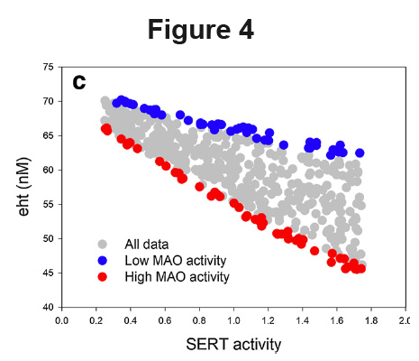 a specific nutrient or vitamin deficiency, and the resulting population can be compared with an untreated population (Nijhout et al., 2017). Not all individuals will respond similarly, and statistical analyses of the two populations can be used to identify genetic make-ups (i.e., specific combinations of parameter values) that make individuals particularly sensitive, or resistant, to the treatment. The parameter makeup of those virtual individuals can then be used to determine which critical values need to be measured in real individuals to identify each subpopulation, and perhaps identify individuals who are likely to be good or bad responders. Here is an example from “Autoreceptor control of serotonin dynamics.” In Figure 4 we show the scatterplot of extracellular serotonin versus SERT activity in a population model where only MAO (monoamine oxidase) activity and SERT activity were varied. High Mao activity is labeled red and low MAO activity is labeled blue. The conclusion is that a selective serotonin reuptake inhibitor (which lowers SERT activity) will have a much greater effect on individuals with high MAO activity than on individuals with low MAO activity because the red line is steeper than the blue line.
The medical importance of the inverse problem. Consider the experiment described in Figure 3 above, or consider the following example. We have three groups of mice, normal mice, obese mice, and depressed mice. The experiment consists of stimulating serotonin release and measuring the concentration of serotonin in the extracellular space over time, after the stimulation, as in Wood et al. (2014) or “Autoreceptor control of serotonin dynamics”. Under repeated trials (repeated mice) for each group one obtains a family of curves. Those families of curves are (somewhat) different for the three groups. One wants to know what that tells us about how the parameters differ between the groups, because that is information about the internal cellular mechanisms that are hard to measure directly. Given a large set of experimental curves, the inverse problem is to use those data to gain information about the distributions of parameters. The traditional methods described in Swigon (2012) cannot be used because those methods assume that variable distributions in the experiment are normal, and that is far from true both in experiments and in our system population models, where we find highly skewed as well as bimodal distributions that cannot be rescaled to normal. So, this question requires new mathematical approaches. Virtual populations produced by system population models can provide a platform for testing such new mathematics, because in such populations everything is known: the topology of the network, the kinetics of the interactions, the values of all parameters, and the values of all variables, for each individual. Because of pervasive nonlinearities in real biological systems, none of the currently available mathematical techniques are able to reconstruct parameters and network topology from the data.
Statistics?? We close by giving an example that shows how difficult it is to draw firm conclusions from statistical analyses. Figure 5 shows scatterplots that relate several metabolites and flux rates in one carbon metabolism, partitioned into two subpopulations with high 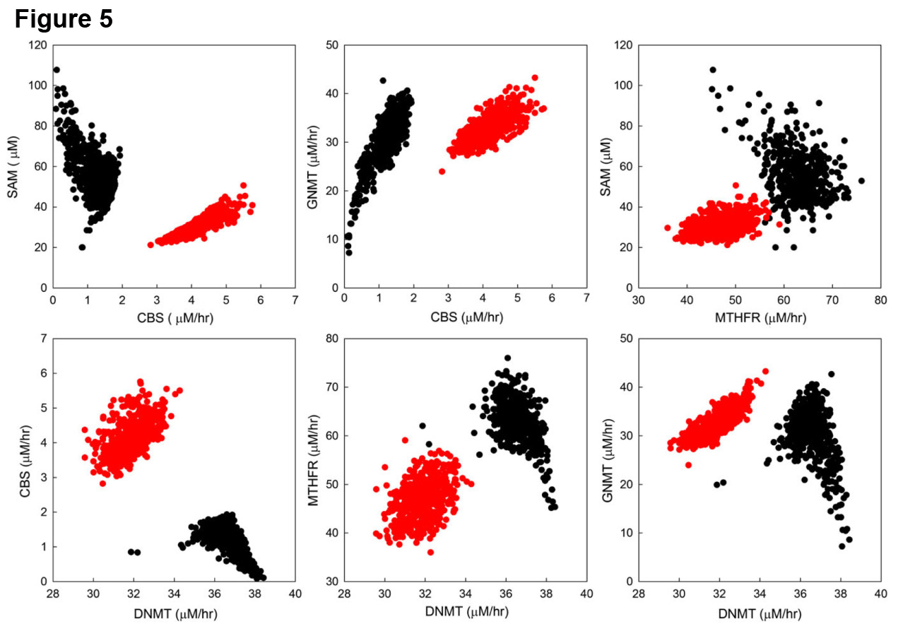 (red) and low (black) blood homocysteine. Homocysteine (Hcy) is a very reactive amino acid that is normally maintained at very low concentrations, and elevated levels of Hcy are recognized as a risk factor for cardiovascular disease (Carmel & Jacobsen, 2001). It is therefore important to understand in what way subpopulations with high and low plasma Hcy levels differ. One can see that each pair of variables is correlated. But the correlations are completely different in the high Hcy subpopulation and the low Hcy subpopulation! This is not an anomaly: the correlations between variables depends on the context in which they are measured. This what one would expect in a highly nonlinear, complicated system, that is crisscrossed by regulatory mechanisms, and serves as a reminder of how difficult it is to understand how biological systems work, and how misleading it can be if one uses a selected subset of a population to deduce parameters for a model. There’s an interesting and difficult issue here, and not just for mathematical modelers. Suppose a biologist measures two variables in rats and finds a correlation. How does she know that those rats are representative and do not come from a special subpopulation?