Category: Srini’s Tech Tips (Page 1 of 6)

Sometimes, the most common method of performing a task is also the least efficient. Commands using menus and ribbon buttons (mouse actions) are convenient and easy, but they also take more time to perform. Here are 5 keyboard shortcuts that can be performed sequentially to create totals and format the numbers to currency style. These shortcuts will increase efficiency and are certainly worth memorizing.

Steps to Perform:

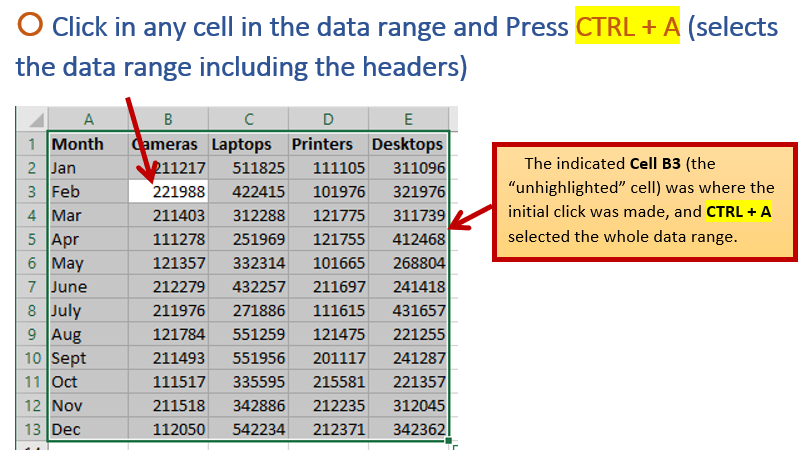
1. Click in the data set, and press CTRL+A (selects all the data, including the headers)
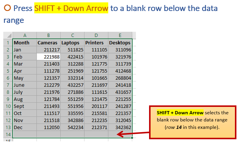
2. Press SHIFT + Down Arrow (Selects the data and a blank row below)
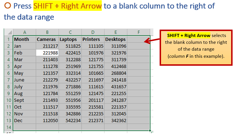
3. Press SHIFT + Right Arrow (Selects the data and a blank column to the right)
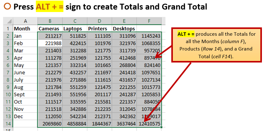
4. Press ALT + = (Creates Totals and a Grand Total)
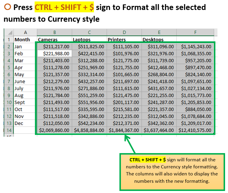
5. Press CTRL + SHIFT + $ sign (Formats the numbers to Currency style)

Click HERE for a practice Excel file to go through these steps yourself.

Screenshots with the Steps Performed:

Many people use Excel efficiently to create reports or provide calculations for analysis.  Most of the time, you may already have data when working with formulas and functions.  However, there are times when you are creating a template / report before the data is available.  Common functions such as SUMS and AVERAGES are very important when doing simple analysis, but missing or unavailable data can lead to formula errors, such as #DIV/0.  The #DIV/0 error is produced when there is missing data, and the average function is dividing by zero or blank.

When an error is produced by formulas or functions, the IFERROR function controls what output value should be displayed in a cell.

The following example shows how you can suppress the #DIV/0 error and display a text message instead, such as “Missing Data”.  A text message is a lot more user-friendly than a formula error.

SYNTAX for IFERROR function:

=IFERROR(value,value_if_error),

Where value is a number or a value resulting from a calculation; value_if_error is the output you want to display when the value or calculation results in an error, such as #DIV/0.  The value_if_error can either be a blank, a number, or text (enclosed in double quotation marks).

EXAMPLE using IFERROR function:

The following example show how the IFERROR function is used to display the words “Missing Data” when the AVERAGE function displays a #DIV/0 error.

• • Figure 1 shows the original AVERAGE function displaying the error.
  • Figure 2 shows how the desired Missing Data message instead of the #DIV/0

Without IFERROR function:

Column G is calculating the average for the people (consultants), however, the missing data is causing the #DIV/0 error.  When the monthly data is entered into the data cells (C6 to E9) the errors will go away.  But, it esthetically more pleasing if the error were suppressed.  The same goes for the Monthly Averages in Row 12.

Formula in Cell G6: =AVERAGE(C6:F6)

Formula in Cell C12: =AVERAGE(C6:C9)

Using the IFERROR function and nesting the AVERAGE function inside

Terminology:  “Nesting” is the term used when you embed a function inside another.

For the YTD Average calculation in Column H, the formula nests the AVERAGE function inside the IFERROR function, but the output “Missing Data” message is displayed (since the AVERAGE function produces a #DIV/0 error).

Formula in Cell H6: =IFERROR(AVERAGE(C6:F6),“Missing Data”)

Similarly, the IFERROR function is also used in Row 16 for the Monthly Averages.

Formula in Cell C16: =IFERROR(AVERAGE(C6:C9),“Missing Data”)

Often you have a table and you only want to extract the data values without all the table formatting.  The common “Copy and Paste Special” or “Paste drop down and select Values” will work, but there is an easier method – right mouse click & drag. While almost everyone understands and uses the left mouse click & drag, mostly for moving objects, many are unaware that you can do a right mouse click & drag technique, which also provides more choices.

Steps: Standard/Common Method

1. Select the data table
2. Click on copy (or CTRL C)
3. Select the destination spot
4. Click on the drop down for paste and choose values (paste icon with 123)

The following example shows how to use the right click & drag method to take the data from a formatted table, and paste just the values, without all the table formatting.  You can perform this action within the same worksheet, or across two separate workbooks, in two separate windows, including two separate monitors.

Steps: Right-Click & Drag Method

1. Select the data table
2. Point your mouse to the right edge of the selection (or any edge you want to move from)
3. When you see the mouse arrow cursor with the 4-way arrow, right click & drag to the desired destination spot (within the sheet or to another workbook sheet in a separate window)

When you release the right mouse button, a menu of options will appear. For this example, select the third option – “Copy Here as Values Only”

• Figure one displays the table and the steps for doing the right click & drag.
• Figure two displays the right click menu that gives you options to choose from.
• Figure three displays the end result of choosing the “values only” option.

Figure 1:  Steps to perform Right-Click & DragFigure 2:  Select the Action option from the Right-click menuFigure 3:  End Result showing Values Copied OnlyAnother Common Use for Right Click and Drag:

• You can right click & drag on a folder or any object, and you can either copy or move the object to the destination spot, without using “copy” or “cut & paste”.
• Below is an example of right-clicking and dragging on a folder. Note you can choose to copy the whole folder (and the contents) – instead of copy & paste.

AutoFilling Large Numbering Series (without manually dragging the AutoFill handle)

You may well be aware of an excellent feature and technique in Excel called AutoFill (covered in the Excel Level 1 course).  The traditional method is that you type the first number in the series, then use the AutoFill handle to drag down to whatever ending number you desire.  While this method is okay for a small series, what happens if you need to number several rows?  The manual dragging method is a cumbersome and quite tedious.

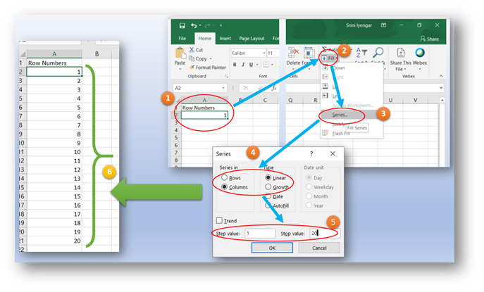
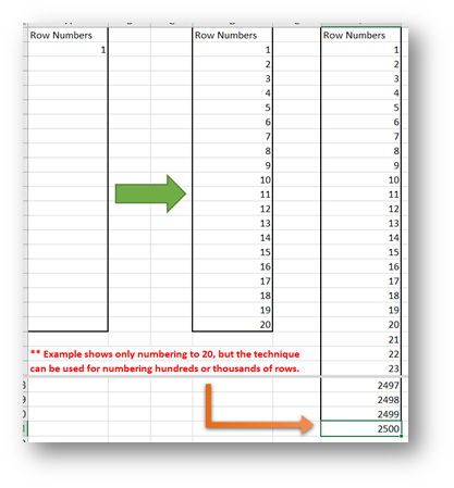
Fortunately, Excel provides an easier method for such a task.  You can use the Fill Series dialog box to enter the sequential number series (aka Linear series), and let Excel fill the row numbers.  The example below illustrates only 20 numbers, but it can easily perform a larger series like in the hundreds or thousands of rows.

NOTE: Steps 1-5 in the illustration are to be performed. Step 6 is the final result.

Steps to Perform:

1. Enter a header for the column, like Row Number (cell A1 in the illustration)
2. Enter the first number and press Enter, but Select the cell again (cell A2 in the illustration)
3. In the Editing group on the Ribbon, click on the Fill drop down
4. Select the Series option from the Fill drop down menu
5. In the Series dialog box, select Columns radio button for series in, and leave the selection as Linear
6. Enter the Ending number in the sequence for the AutoFill (the illustration shows 20 as the ending number, but you can enter a higher ending number)
7. Click OK (Excel now has entered all the row numbers from 1 to the Ending Number).

NOTE: The illustration shows AutoFilling for 2500 rows.