Given that sports betting has come to North Carolina I am going to revisit the topic and derive some general formulas. The take home message is that while you might think you could make money betting against people who know less than you do. It is just like going to a casino.  The typical moneyline wager looks like

Fav(orit)e  -B      (Under)Dog +A

What this means is that you have to bet $B on Fave to win $100, while if you bet $100 on Dog you win $A. Let p be the probability Dog wins.

For the bet on Fave to be fair we need 100(1-p) – Bp = 0 or p = 100/(100+B)

For the bet on Dog to be fair we need -100(1-p) + Ap= 0 or p = 100/(100+A)

In practice A< B so if 100/(100+B) < p < 100/(100+A) both bets are unfavorable.

For a numerical example, in the sweet 16 of the 2024 NCAA tournament we saw the bet

Marquette -300, NC State + 230, so both are unfavorable if

0.25 = 100/400 < p < 100/330 = 0.303

In this particular case NC State won, which is not incredibly unexpected since when you roll two dice then the probability of a total of 9 or more has probability 10/36 = 0.2777

Another way of looking at this is through the money bet. If a fraction x of people bet on Fave then

When Fave wins the average winnings are 100x – 100(1-x) which is < 0 if x < 1/2

When Dog wins the average winnings are -B x + A(1-x) which is < 0 if x > A/(A+B)

In our concrete example both bets are bad for players if 0.434 = 230/530 < x < 1/2

While the sports book has no control over the probability that Dog wins, they can control the fraction of money bet on the favorite by adjusting the odds over time, or using their knowledge of previous bets to choose good values of A and B.

When A/(A+B) < x < ½ then the sports book has an arbitrage opportunity. They will make money under either outcome. In the theory of option pricing it is assumed that arbitrage opportunities do not exist (or if they do are short lived), and based on this one can derive what is the right price for a “derivative security” such as a call or put option based on the stock prices.

If you want to learn about this look at Chapter 6 of my book Essentials of Stochastic Processes which you can download in pdf form from my web page. https://services.math.duke.edu/~rtd/EOSP/eosp.html

My goal here is to make two points (i) the sports books are not gambling: they have things set up so that they win money no matter what the outcome is, (ii) even though you are gambling against a group of people and it seems that you can win money if you are smarter than they are, that is an illusion. Like casino gambling, things are set up so that all of the bets are unfavorable. So like the TV commercials say look at sports betting as a way of enhancing the fan experience not as a way to make money. However with betting available 24-7, in game parlays and bonus bets designed to get you used to betting a lot of money, this like the lottery, is a scheme designed to take money from people who are gambling with money they can’t afford to lose.

My first job was at UCLA in 1976. The legendary Ted Harris who wrote one of the first books on branching processes, found a tractable subset of Markov chains on general state space that bears his name, and invented the contact process was there at University of Southern California. USC was only about 20 miles away and Ted Cox was there from 1977-1979, so I would often go over there on Friday afternoon for the probability seminar. On weeks when there was an outside speaker, Ted and his wife Connie would have little after-dinner desert parties in their house at the southeastern edge of Beverly Hills. One of Connie’s favorite things to say was, you guessed it, “There is no such thing as probability.” To support this claim she would tell stories in which something seemingly impossible happened. For example, one evening after eating at a restaurant, she realized while walking to the exit that she had left her purse at the table. She went back to the table to retrieve it and along the way saw an old friend that she had not seen in many years. She would never had seen the friend unless she had forgotten her purse. The punch line of the story was “What is the probability of that?”

The connection with basketball is that this year’s March Madness seems to violate some of the usual assumptions of probability.

The probability of events such as black coming up on a roulette wheel do not change in time. Of course, the probability a team wins a game depends on their opponent, but we don’t expect that the characteristics of the team will change over time. This is false for this year’s Duke Blue Devils. They lost to UNC in coach K’s retirement game on March 5, and sleepwalked their way through the ACC tournament needs late game surges to beat Syracuse and Miami, before losing to Virginia Tech in the finals.

They won their first game in the NCAA against Cal State Fullerton. This was a boring game in which the difference in scores being like the winnings of  a player betting on black every time. Playing against Michigan State, it looked like it was all over when Duke was down by 5 with a minute to play but they rallied to win. In the next game against Texas Tech in a late game time out, the players convinced coach K to let them switch from zone defense to man-to-man. If I have the story right, at that moment coach K slapped the floor, and then the five players all did so simultaneously, an event of intense cosmic significance, and Texas Tech was done for. Maybe the French theory of grossissement de filtration can take account of this, but I am not an expert on that.

You have to take account of large deviations. In the first round #15 seed St. Peter’s stunned the nation with an upset victory over #2 Kentucky, and then beat #7 Murray State to reach the Sweet 16 where they played Purdue. St. Peters plays with four guards and early in the game substituted five new players for the starting five. The four guards buzzed around the court annoyed the players that were bringing the ball up the floor and generally disrupted Purdue’s game. To the 7’4” center they were probably like the buzzing of bees that he could hear but not see since they were so far below him.

Basketball is a great example of Lévy’s 0-1 law: the probability of a win, an event we’ll call W, given the current information about the game (encoded in a sigma field F_t) converges to 0 or 1 as t tends to ꝏ (which is usually 40 minutes but might include over time). Late in the game this quantity can undergo big jumps. Purdue was down by 6 with about a half-minute to play and desperately needed a three point shot. The player with the ball turned to throw it to a player who he thought would be nearby and open, only to find that the player had decided to go somewhere else, and suddnely the probability dropped much closer to 0

Games are not independent. Of course, the probability a team wins a game depends on their opponent, but even if you condition on the current teams, the tournament does not have the Markov property. On Thursday March 24 Arkansas upset #1 seed Gonzaga. After this emotional win and with little time to prepare they played Duke on Saturday and slowly succumbed. In a display of coach K’s brilliance “Duke won the final minute of the first half” increasing their lead from 7 points to 12. Even though the game was a martingale after the end of the first half, the L² maximal inequality guaranteed than a win was likely.

The high point of the Duke-Kansas game came about two minutes into the second half when an Arkansas three point shot bounced off the rim and ended resting on top of the backboard. A quick thinking (and very pretty) Arkansas cheerleader got up on the shoulder of her male partner for their gymnastic routines. Putting her two little pom-poms in one hand she reached up and tipped the ball back down to the floor.

To end where I began What is the probability of that? To use the frequentist approach we can count the number of games in the regular season and in the tournament in which this event occurred and divide by the number of games. The answer would be similar the Bayesian calculation that the sun will rise tomorrow. Using Google and using the curious biblical assumption that the solar system is 5000 years old gives (as I read on the internet) that the probability that the sun will not rise today is 1/186,215. Even though it may seem to my wife that there are this many games, I have to agree with Connie Harris: in March Madness there is no such thing as probability.

It has been 18 months since my last blog post. At that point I was very angry about Trump’s mishandling of the covid pandemic and the fact that people wouldn’t wear masks, while on other days I was saying goodbye to two former colleagues who were mentors, colleagues, and good friends. Not much has changed: now I am angry about people who won’t get vaccinated and I spend my time sticking pins into my Aaron Rodgers voodoo doll hoping that a covid outbreak on his team will keep him from winning the Super Bowl.

To calm myself I have decided to do some math and relax. It is a well-known result (but not easy for an impatient person to find on the internet) that if you are playing a game that is biased against, bold play is optimal. Specifically, if  you want to reach a fixed target amount of money when playing such a game then the optimal strategy is to bet all the money you have until you reach the point where winning will take you beyond your goal and then bet only enough to reach your goal.

For a concrete example, suppose (i) you have $1 and your wife wants you to take her from brunch at the Cheesecake Factory which will cost you $64, and (ii) you want to win the necessary amount of money by betting on black at roulette where you win $1 with probability 18/38 and lose $1 with probability 20/38. A standard calculation, which I’ll omit since it is not very easy to type in Mircosoft Word, (see Example 1.45 in my book Essentials of Stochastic Processes) shows that the probability I will succeed is 1.3116 x 10 ^-4. In contrast the strategy of starting with $1 and “letting it ride” with the hope that you can win six times in a row has probability (18/38)⁶ = 0.01130. This 86 times as large as the previous answer, but still a very small probability.

Consider now the NFL football game between the Green Bay Packers and the Baltimore Ravens held on Sunday December 19, 2021. After trailing 31-17 the Ravens scored two touchdowns to bring the score to 31-30. To try to win the game without going to overtime they went for a two-point conversion, failed and lost the game. Consulting google I find that surprisingly 49.4% of two point conversions are successful versus 94.1% of kicks for one point. In this game under consideration the two point conversion would not necessarily win the game, since there were about 45 seconds left on the clock with Green Bay having one time out, so there is some chance (say 30%) that Green Bay could use passes completed near the sideline to get within range to make a field goal and win the game 34-32. Rounding 49.4 to 50, going for two results in a win probability for the Ravens of 35%. With a one-point conversion their win probability is 0.94 x 0.7 x p, where p is the probability of winning in overtime. If p = ½ this is 33%. However, if the 8-6 Ravens feel like the 11-3 Packers have a probability significantly bigger than ½ to win in overtime then the right decision was to go for two points.

A second example is provided by the Music City Bowl game between Tennessee and Purdue, held December 30, 2021. After a fourth quarter that saw each team score two touchdowns in a short amount of time (including a two-point conversion by Purdue to tie the score), each had 45 points. The pre-overtime coin flip determined that Tennessee would try to score first (starting as usual from the opponent’s 25 yard line). Skipping over the nail biting excitement that makes football fun to watch, we fast-forward to Tennessee with fourth down and goal on the 1 yard line. The timid thing to do would be to kick the field goal which has a probability that is essentially 1. In this case if Purdue

(i) scores a touchdown (with probability p7) Tennessee (or T for short) loses

(ii) kicks a field goal (with probability p3), they go to a second overtime period

(iii) does not score (with probability p0) T wins

Using symmetry the probability T wins is p0 + p3/2 = 1 – p7 – p3/2

Case 1. If T fails to score (which is what happened in the game) then the Purdue will win   with high probability, since they only need a field goal. In the actual game, three running plays brought the ball 8 yards closer and then the kicker made a fairly routine field goal.

Case 2. If T scores (with probability q) then Purdue must score a touchdown, an event of probability P7 > p7 so the probability T wins when they try to score a touchdown is q[(1-P7) +P7/2]

There are a few too many unknowns here, but if we equate p7 with scoring a touchdown when the team is in the red zone (inside the 20) then the top 10 ranked teams all have probabilities of > 0.8. If we take q=0.5, set p7=0.8 then the probability T wins in Case 2 is 0.3 versus 0.2 – p3/2 in Case 1 which is 0.15 if p3=0.1 (half the time they don’t score a touchdown they get a field goal.

Admittedly like a student on exam with a question they don’t know the answer to, I have laid down a blizzard of equations in hopes of a better score on the problem. But in simple terms since p7 is close to 1, the Tennessee coach could just skip all the math and assume Purdue would go on to score a touchdown on their possession and realize he needs his team to score a touchdown, which regrettably they did not.

Like many posts I have written, the story ended differently than I initially thought but you have to follow the math where it takes you.

With the orange jackass (aka widdle Donnie) first declaring the coronova virus a hoax, then telling people to go ahead and go to work if you are sick, and only today tweeting that the people at the CDC are amazed at how much he knows about covid-19, it is time to have some fun.

Tonight (March 7) at 6PM in Cameron Indoor Stadium the Blue Devils with a conference record of 14-5 will take on the UNC Tarheels  who are 6-13 and will end up in lst place if they lose. If you go online to look at the odds for tonight’s Duke-UNC you find the curious looking

Duke -350

UNC 280

What this means is that you have to bet $350 on Duke to win $100, while if you bet $100 on UNC you win $280

Let p be the probability Duke wins.

For the bet on Duke to be fair we need 100p – 350(1-p) = 0 or p = 7/9 = 0.7777

For the bet on UNC to be fair we need -100p + (1-p)280= 0 or p = 0.7368

If 0.7368 < p < 0.7777 both bets are unfavorable.

This suggests that the a priori probability Duke wins is about 3/4.

Another way of looking at this situation is through the money. If a fraction x of people bet on Duke then

When Duke wins the average winnings are 100x – 100(1-x)

When UNC wins the average winnings are -350 x + 280 (1-x)

Setting these equal gives 200 x + 630 x = 100 + 280 or x = 38/83 = 0.4578

If this fraction of people bet on Duke then the average payoff from either wager is -500/83 = -$6.02 and the people who are offering the wager don’t care who wins.

Harry Kesten at Cornell in 1970 and in his later years

On March 29, 2019 Harry Kesten lost a decade-long battle with Parkinson’s disease. His passing is a sad event, so I would like to find solace in celebrating his extraordinary career. In addition I hope you will learn a little more about his work by reading this.

Harry was born in Duisburg Germany on November 19, 1931.  His parents escaped from the Nazis in 1933 and moved to Amsterdam. After studying in Amsterdam, he was a research assistant at the Mathematical Center there until 1956 when he came to Cornell. He received his Ph.D. in 1958 at Cornell University under supervision of Mark Kac.

In his 1958 thesis on Symmetric Random Walks, he showed that the spectral radius equals the exponential decay rate of the return to 0, and the latter is strictly less than 1 if and only if the group is non-amenable  This work has been cited 206 times and is his second most cited publication (according to MathSciNet). Harry was an instructor at Princeton University for one year and at the Hebrew University for two years before returning to Cornell, where he spent the rest of his career. While in Israel, he and Furstenberg wrote their classic paper on Products of Random Matrices.

In the 1960s, he wrote a number of papers that proved sharp or very general results on random walks, branching process, etc. One of the most famous of these is the 1966 Kesten-Stigum theorem which shows that a a normalized branching process Z_n/μⁿ has a nontrival limit if and only if the offspring distribution has E(X log⁺ X) < ∞.  In 1966 he also proved a conjecture of Erdös and Szuzu about the discrepancy between the number of rotations of a point on the unit circle hitting an interval and its length. Foreshadowing his work in physics, he showed in 1963 that the number of self-avoiding walks of length n satisfied σ_n+2/σ_n → μ² , where μ is the connective constant.

Harry’s almost 200 papers have been cited 3781 times by 2329 authors However, these statistics underestimate his impact. In baseball terms, Harry was a closer. When he wrote a paper about a topic, his results often eliminated the need for future work on it. One of Harry’s biggest weaknesses is that he was too smart. When most of us are confronted with a problem, we need to try different approaches to find a route through the woods to a solution. Harry simply got on his bulldozer and drove over all obstacles. He needed 129 pages in the Memoirs of the AMS to answer the question: “Which processes with stationary independent increments hit points?”, a topic he spoke about at the International Congress at Nice in 1970.

In 1984 Harry gave lectures on first passage percolation at the St. Flour Probability Summer School. This subject dates back to Hammersley’s 1966 paper and was greatly advanced by Smythe and Weirman’s 1978 book. However, Harry’s paper attracted a number of people to work on the subject and it has continued to be a very active area. See 50 years of First Passage Percolation by Auffinger, Damron, and Hanson for more details. You can buy this book from the AMS or download it from the arXiv.  I find it interesting that Harry lists only six papers on his Cornell web page. Five have already been mentioned. The sixth is On the speed of convergence in first-passage percolation, Ann. Appl. Probab. 3(1993), 296–338.

Harry has worked in a large number of areas. There is not enough space for a systematic treatment so I will just tease you with a list of titles. Sums of stationary sequences cannot grow slower than linearly. Random difference equations and renewal theory for products of random matrices. Subdiffusive behavior of a random walk on a random cluster. Greedy lattice animals. How long are the arms of DLA? If you want to try to solve a problem Harry couldn’t, look at his papers on Diffusion Limited Aggregation.

In the late 1990s, Maury Bramson and I organized a conference in honor of Harry’s 66 2/3’s  birthday. (We missed 65 and didn’t want to wait for 70.) A distinguished collection of researchers gave talks and many contributed to a volume of papers in his honor called Perplexing Problems in Probability. The 21 papers in the volume provide an interesting snapshot of research at the time. If you want to know more about Harry’s first 150 papers, you can read my 32 page summary of his work that appears in that volume.

According to math genealogy, Harry supervised 17 Cornell Ph.D. students who received their degrees between 1962-2003. Maury Bramson and Steve Kalikow were part of the Cornell class of 1977 that included Larry Gray and David Griffeath who worked with Frank Spitzer. (Fortunately, I graduated in 1976!). Yu Zhang followed in Harry’s footsteps and made a number of contributions to percolation and first passage percolation. I’ll let you use google to find out about the work Kenji Ichihara, Antal Jarai, Sungchul Lee, Henry Matzinger, and David Tandy.

Another ‘broader impact” of Harry’s work came from his collaborations with a long list of distinguished co-authors: Vladas Sidorovicius (12 papers), Ross Maller (10) , Frank Spitzer (8), Geoffrey Grimmett (7), Yu Zhang (7), Itai Benjamini (6), J.T. Runnenberg (5), Roberto Schonmann (4), Rob van den Berg (4), … I wrote 4 papers with him, all of which were catalyzed by an interaction with another person. In response to a question asked by Larry Shepp, we wrote a paper about an inhomogeneous percolation which was a precursor to work by Bollobas, Janson, and Riordan. Making money from fair games, joint work with Harry and Greg Lawler, arose from a letter A. Spataru wrote to Frank Spitzer. I left it to Harry and Greg to sort out the necessary conditions.

Harry wrote 3 papers with two very different versions of Jennifer Chayes. With a leather-jacketed Cornell postdoc, her husband Lincoln Chayes, Geoff Grimmett and Roberto Schonmann, he studied “The correlation length for the high density phase.” With the manager of the Microsoft research group, her husband Christian Borgs, and Joel Spencer he wrote two papers, one on the birth of the infinite component in percolation and another on conditions implying hyperscaling.

As you might guess from my narrative, Kesten received a number of honors. He won the Brouwer medal in 1981. Named after L.E.J. Brouwer it is The Netherlands’ most prestigious award in mathematics. In 1983 he was elected to the National Academy of Science. In 1986 he gave the IMS’ Wald Lectures. In 1994 he won the Polya Prize from SIAM. In 2001 he won the AMS’ Steele Prize for lifetime achievement.

Being a devout orthodox Jew, Harry never worked on the Sabbath. On Saturdays in Ithaca, I would often drive past him taking a long walk on the aptly named Freese Road, lost in thought. Sadly Harry is now gone, but his influence on the subject of probability will not be forgotten.

My last two posts were about a hurricane and a colonscopy, so I thought it was time to write about some math again.

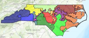
For the last five years Mattingly has worked on a problem with important political ramifications: what would a typical set of congressional districts (say the 13 districts in North Carolina) look like if they were chosen at “random” subject to the restrictions that they contain a roughly equal number of voters, are connected, and minimize the splitting of counties. The motivation for this question can be explained by looking at the current congressional districts in North Carolina. The tiny purple snake is district 12. It begins in Charlotte goes up I40 to Greensboro and then wiggles around to contain other nearby cities producing a district with a large percentage of Democrats.

To explain the key idea of gerrymandering, suppose, to keep the arithmetic simple, that a state has 2000 Democrats and 2000 Republicans. If there are four districts and we divide voters

District           Republicans       Democrats

1                           600                            400

2                           600                            400

3                           600                            400

4                           200                            800

then Republicans will win in 3 districts out of 4. The last solution extends easily to create 12 districts where the Republicans win 9. With a little more imagination and the help of a computer one can produce the outcome of the 2016 election in North Carolina election in which 10 Republicans and 3 Democrats were elected, despite the fact that the split between the parties is roughly 50-50.

The districts in the North Carolina map look odd, and the 7th district in Pennsylvania (named Goofy kicks Donald Duck) look ridiculous, but this is not proof of malice.

Mattingly with a group of postdocs, graduate students, and undergraduates has developed a statistical approach to this subject. To explain this we will consider a simple problem that can be analyzed using material taught in a basic probability or statistics class. A company has a machine that produces cans of tomatoes. On the average the can contains a pound of tomatoes (16 ounces), but the machine is not very precise, so the weight has a standard deviation (A statistical measure of the “typical deviation” from the mean) of 0.2 ounces. If we assume the weight of tomatoes follows the normal distribution then 68% of the time the weight will be between 15.8 and 16.2 ounces. To see if the machine is working properly an employee samples 16 cans and finds an average weight of 15.7 pounds.

To see if something is wrong we ask the question: if the machine was working properly then what is the probability that the average weight would be 15.7 pounds or less. The standard deviation of one observation is 0.2 but the standard deviation of the average of 16 observations is 0.2/(16)^1/2  = 0.005. The observed average is 0.3 below the mean or 6 standard deviations. Consulting a table of the normal distribution or using a calculator we see that if the machine was working properly then the probability of an average of 15.7 or less would occur with probability less than 1/10,000.

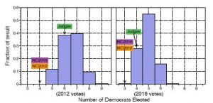
To approach the gerrymandering, we ask a similar question: if the districts were drawn without looking at party affiliation what is the probability that we would have 3 or fewer Democrats elected? This is a more complicated problem since one must generate a random sample from the collection of districts with the desired properties. To do this Mattingly’s team has developed methods to explore the space of possibilities and then making successive small changes in the maps. Using this approach one has make a large number of changes before you have a map that is `independent.” In a typical analysis they generate 24,000 maps. They found that using the randomly generated maps and retallying the votes, ≤3 Democrats were elected in fewer than 1% of the scenarios. The next graphic shows results for the 2012, 2016 maps and one drawn by judges.

Mattingly has also done analyses of congressional districts in Wisconsin and Pennsylvania, and has helped lawyers prepare briefs for cases challenging voting. His research has been cited in many decisions including the three judge panel who ruled in August 2018 that the NC congressional district were unconstitutional. For more details see the Quantifying Gerrymandering blog

https://sites.duke.edu/quantifyinggerrymandering/author/jonmduke-edu/

Articles about Mattingly’s work have appeared in

(June 26, 2018) Proceedings of the National Academy of Science 115 (2018), 6515–6517

(January 17, 2018)  Nature 553 (2018), 250

(October 6, 2017) New York Times  https://www.nytimes.com/2017/10/06/opinion/sunday/computers-gerrymandering-wisconsin.html

The last article is a good (or perhaps I should bad) example of what can happen when your work is written about in popular press. The article, written by Jorden Ellenberg is, to stay within the confines of polite conversation, simply awful. Here I will confine my attention to its two major sins.

1. Ellenberg refers several times to the Duke team but never mentions them by name. I guess our not-so-humble narrator does not want to share the spotlight with the people who did the hard work. The three people who wrote the paper are Jonathan Mattingly, professor and chair of the department, Greg Herschlag, a postdoc, and Robert Ravier, one of our better grad students. The paper went from nothing to fully written in two weeks in order to get ready for the court case. However, thanks to a number of late nights they were able to present clear evidence of gerrymandering. It seems to me that they deserve to be mentioned in the article, and it should have mentioned that the paper was available on the arXiv, so people could see for themselves.
2. The last sentence of the article says “There will be many cases, maybe most of them, where it’s impossible, no matter how much math you do, to tell the difference between innocuous decision making and a scheme – like Wisconsin’s – designed to protect one party from voters who might prefer the other.” OMG. With many anti-gerrymandering lawsuits being pursued across the country, why would a “prominent” mathematician write that in most cases math cannot be used to detect gerrymandering?

Today is January 7, 2018. I am tired of Trump bragging that he is a “very stable genius.” Yes he made a lot of money (or so he says) but he doesn’t know what genius looks like. Today’s column is devoted to work of Wesley Pegden (and friends) on the Abelian Sand Pile Model. Why this topic. Well he is coming to give a talk on Thursday in the probability seminar.

This system was introduced in 1988 by Bak, Tang, and Wiesenfeld (Phys Rev A 38, 364).  The simplest version of the model takes place on a square subset of the two dimensional integer lattice. Grains of sand are dropped at random. The number of grains at a point is ≥ 4 the pile topples and one grain is sent to each neighbor. This may cause other sites to topple setting off an avalanche.

The word Abelian refers to the property that the state after n grains have landed is independent of the order in which they are dropped. The reason that physicists are interested is that the system “self-organizes itself into a critical state” in which avalanche sizes have a power law. The Abelian sand pile has been extensively studied, and there are connections to many branaches of mathematics, but for that you’ll have to go to the Wikipedia page or to the paper “What is … a sandpile?” written by Lionel Levine and Jim Propp which appeared in the Notices of the AMS 57 (2010), 976-979.

In a 2013 article in the Duke Math Journal [162, 627-642] Wesley Pegden and Charles Smart studied what happened when you put n grains of sand at the origin on the infinite d-dimensional lattice and let the system go until it reaches its final state. They used PDE techniques to show that when space is scaled by n ^1/d then the configuration converges weakly to a limit, i.e, integrals against a test function converge. As Fermat once said the proof won’t fit in the margin, but in a nutshell what they do is to who used viscosity solution theory to identify the continuum limit of the least action principle of Fey–Levine–Peres (J. Stat. Phys. 138 (2010), 143-159). A picture is worth several hundred words.

In a 2016 article in Geometric and Functional Analysis, Pegden teamed up with Lionel Levine (now at Cornell) to study the fractal structure of the limit. The solution is somewhat intricate involving solutions of PDE and Apollonian triangulations that generalize Apollonian circle packings.

References

Mutesa, L et al (2020) A strategy for finding people infected with SARS-CoV-2: optimizing pooled testing at low prevalence arXiv: 2004.14934
Malliapaty, Smriti (2020) The mathematical strategy that could transform coronavirus testing. Nature News July 10. https://www-nature-com/articles/d41586-020-02053-6
Moneyline Wagering