
Background
Our idea of this robot stems from the tournament – Robomaster NA. In this tournament, universities across the entire states and even the globe bring their own customized robots and play FPS in an enclosed venue. What we are trying to do in this capstone class is to develop some techniques that are transferable to our team and will probably have some innovation in our next-gen infantry robots.
In recent years, most university teams have still used traditional configurations such as Mecanum and Omni wheel for drive chain. These have their own advantages, such as agility and chassis rotation capabilities. However, with the increasing changes in competition rules, the arena is no longer simply flat ground, but includes more slopes and bumpy road. This poses a greater challenge to the robot’s maneuverability.
On the other hand, the competition committee has also begun to encourage teams to build other new chassis configurations, such as the balanced chassis. The new rules also provide significant advantages, for example, the balanced robot can have higher chassis power and buffer energy during competitions. This provides us with a great deal of motivation and demand for developing new balancing robots in the future season.
Problem Statment
Current balanced robot design are easily dominated by uneven terrain, resulting in poor robot mobility. A novel balancing robot design features a bipedal wheel–legged configuration that combines high energy efficiency with strong terrain adaptability. Unlike traditional segway and inverted-pendulum robots that rely on closed-chain 5-bar mechanisms, our robot uses an open-chain leg structure, enabling self-rescue and greater adaptability during motion.
Project Objectives
For this project, our primary objective is to verify the feasibility of the open-chain wheel-legged balancing robot and the following development:
- Verify the basic inverted pendulum balancing cart demo.
- Finish the mechanical design of an open-chain five-bar linkage wheel-leg robot.
- Analyze the locomotion of the wheel-leg robot and explore the function of the Linear Quadratic Regulator controller.
- Build a single-leg test platform to implement the standing function.
By achieving these goals, we hope to provide future team members with a design foundation, helping them better understand the design process and develop our own balancing robot for competitions.
Education Objective
- Develop proficiency in advanced SolidWorks sketching techniques for the design of complex linkages and motor output structures.
- Learn to process IMU sensor data using appropriate filtering methods for reliable state estimation.
- Explore embedded system development by implementing and evaluating CAN bus communication on a new hardware platform.
- Analyze and compare LQR and PID control strategies, supported by MATLAB/Simulink simulations to evaluate system performance.
Research Objective
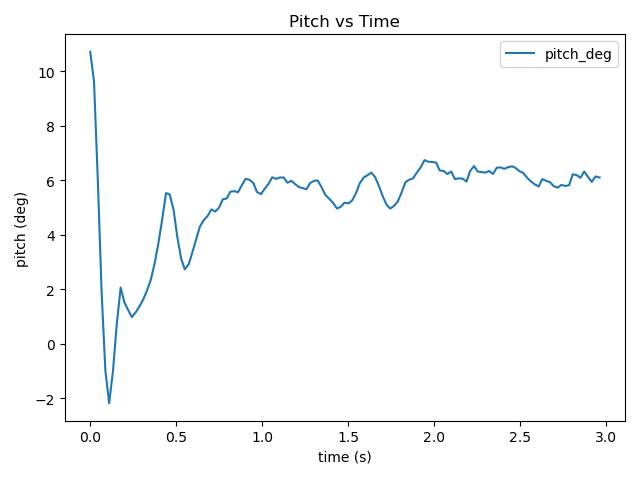
This project focuses on the design and dynamic analysis of a new type of leg cooling system, as well as the modeling of balance control and chassis attitude calculation. The robot’s configuration should be able to overcome bumpy roads and have some obstacle-crossing capabilities. Furthermore, the pitch angle of the robot’s chassis should not exceed a certain angle throughout the entire movement. Finally, the robot should be able to self-rescue and reset its chassis when it tipps over.
Design Matrix
Project Decomposition:

Milestones:

The IMU (Inertial Measurement Unit) serves as the critical ‘inner ear’ for a two-wheeled self-balancing robot. It captures essential data on angular velocity and acceleration to estimate the robot’s tilt angle (pitch).
However, raw sensor signals are subject to noise and drift. Currently, the mainstream filtering algorithm for balance cars is Complementary Filtering. While this method is intuitive, its reliance on fixed parameters makes it unable to adapt to varying noise or dynamic environmental conditions.
Theoretically, the balance robot can be regarded as a pendulum with no friction and with instantaneous motor response. However, practical challenges include battery voltage fluctuations, unstable mechanical center of gravity, sensor noise, and electronic component installation issues (e.g., MPU6050 pins not properly soldered on the circuit board, causing significant sway that affects attitude angles). Therefore, his work focuses on making a reliable balance robot model, implementing robust filtering algorithms to fuse the IMU data. Since two-wheeled balance robot and bipedal-wheeled robot are essentially in the class of pendulum model, his work will verify the effectiveness of the more robust filtering algorithm, which is the foundation for the control system to maintain the future bipedal-wheeled robot’s dynamic stability.
- Building Experimental Platform
Step 1: Connectivity test
At the beginning he chose ESP32 as circuit board, MPU6050 as IMU, connected on a breadboard, and tested on PlatformIO in VSCode. The output data is shown in VSCode terminal in Fig 1. This step is to test if IMU is connected to microcontroller.
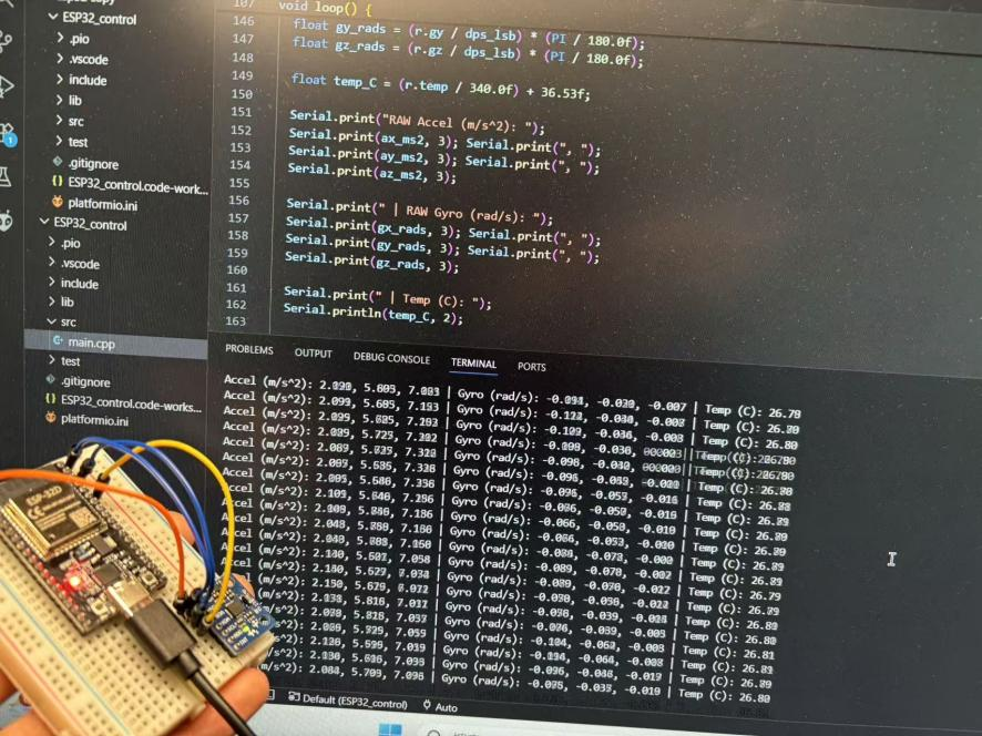
Fig 1 raw data output in VSCode
He wrote a script to visualize Roll-Pitch-Yaw data, so that when the breadboard is tilted in different directions, wave form makes corresponding changes, as shown in Fig 2. Note that data is sent to a webpage by WiFi, so time delay is normal. When the IMU later connect to the circuit board, time delay can be ignored. This step is to test if IMU is working normally, and if the data is reasonable. If so it is expected to be responsive to tilting, and the waveform should exhibit corresponding oscillations, including amplitude, angle class and direction. To further explain this, when the breadboard tilts about y-axis, It is expected to see the curve corresponding to Pitch angle oscillates most heavily, the heavier tilt the breadboard has, the larger the amplitude of the curve should be, counterclockwise and clockwise tilting should relate to two sides of the curve.
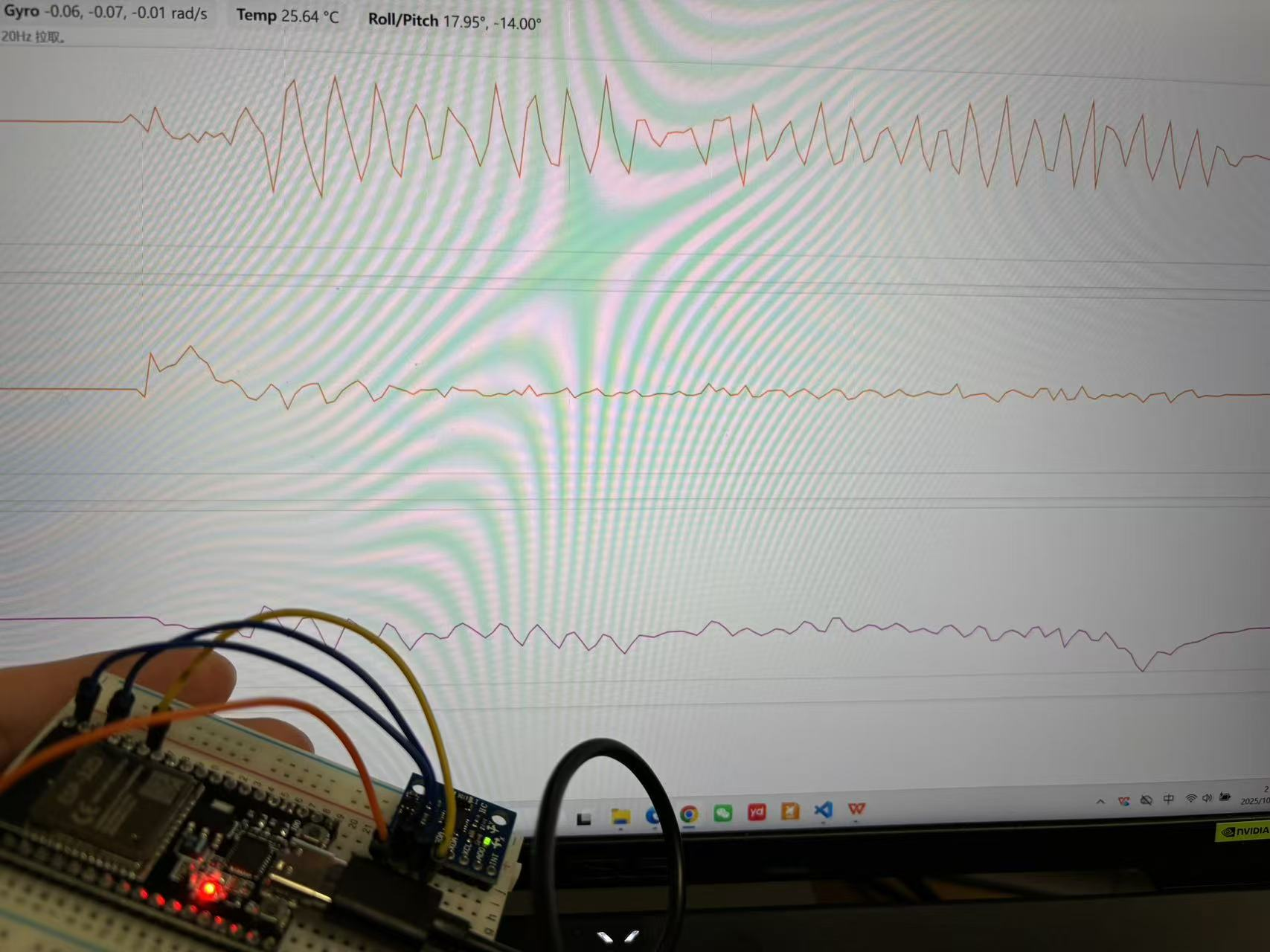
Fig 2 Visualization of RPY angles
Step 2: IMU-motor test
To test if IMU data can be applied onto motor successfully, he wrote a script that control a stepper motor rotating direction using pitch angle, as shown in Fig 3. When the IMU tilts forward, the motor rotates forward; when tilting backward, the motor rotates backward.

Fig 3 IMU data applied on motor test
Step 3: Prototyping
Merely aligning the motor direction with the tilt angle is insufficient. To validate the effectiveness of the filtering algorithms, he prototyped a self-balancing robot. The process is outlined below.
He chose two TT DC motors (with wheels), Elegoo Nano V3 as microcontroller, MPU6050 as IMU, TB6612FNG as motor driver, a 6v battery pack, and a breadboard, as shown in Fig 4.

Fig 4 *Pictures are all from Google Images.* (from left to right) TT DC motors (with wheels), Elegoo Nano V3, MPU6050, TB6612FNG, a 6v battery pack, a breadboard.
The breadboard was adhered to the robot chassis. The only thing that needs to pay attention to is the position of each module. He assembled them together so that its center of mass is in the same plane that goes across two wheels’ centers. It ensures that when placed properly, the robot should be at static balance, which makes dynamic balancing feasible.
The final product is shown in Fig 5.
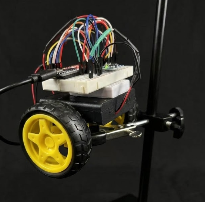
Fig 5 two-wheeled self balancing robot
- Experiment Design
The goal is to compare the performance between no filter, Complementary Filter and Adaptive Complementary Filter. Raw IMU signals are imperfect: accelerometers suffer from high-frequency noise due to vibrations, while gyroscopes accumulate drift over time. Filtering is essential to fuse these signals, combining long-term accelerometer stability with short-term gyroscope precision for an accurate angle estimate. A standard complementary filter uses a fixed gain to merge these signals. In contrast, an adaptive complementary filter dynamically adjusts this gain based on real-time motion conditions, such as total acceleration.

From CF to ACF, coefficient alpha switches from a fixed one alpha, to a time-dependent one alpha_k. The advantage of the adaptive approach is improved robustness during dynamic situations. By automatically reducing reliance on the accelerometer when external acceleration is detected, it prevents large angle errors during fast movements while remaining computationally simple.[1]
To verify this , he set three scenarios altogether. Two scenarios are common in a real world robot running case and one static scenarios, which are static, slow motion, forward. The experimental setup is illustrated in Fig 6 and Fig 7.
Fig 6 Robot on a stand
Fig 6 shows the setup for static scenario. The robot is held on a stand so it’s static.
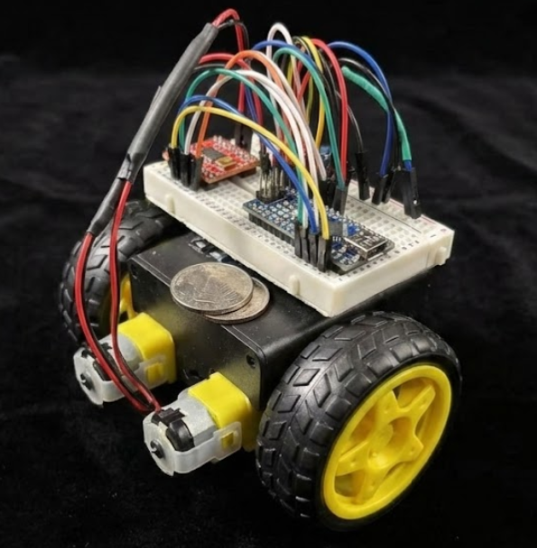
Fig 7 Robot on desk
Fig 7 shows the setup for slow motion and forward scenarios. Notice that two coins are placed on the robot so that when it’s released it will go forward because of the effect of coin mass. The coins are glued and there is a cable connected to his laptop in real tests.
- Videos:
CF:
ACF:
- Data Analysis
For each scenario, he conducted the experiment for unfiltered, CF and ACF, generating 4 figures for each filter case (Pitch, Roll, Gyro, Accelerometer). That would be 3*3*4=36 figures in total. In a robot balancing case, Pitch angle and gyro are the most important to focus since they make more sense in keeping balance. Also to some extent in order to keep the website concise, only Pitch and Gyro figures in each case are selected and put on the website.
1.Static (from left to right, Unfiltered, CF, ACF, applied to all)
-Pitch
-Gyro
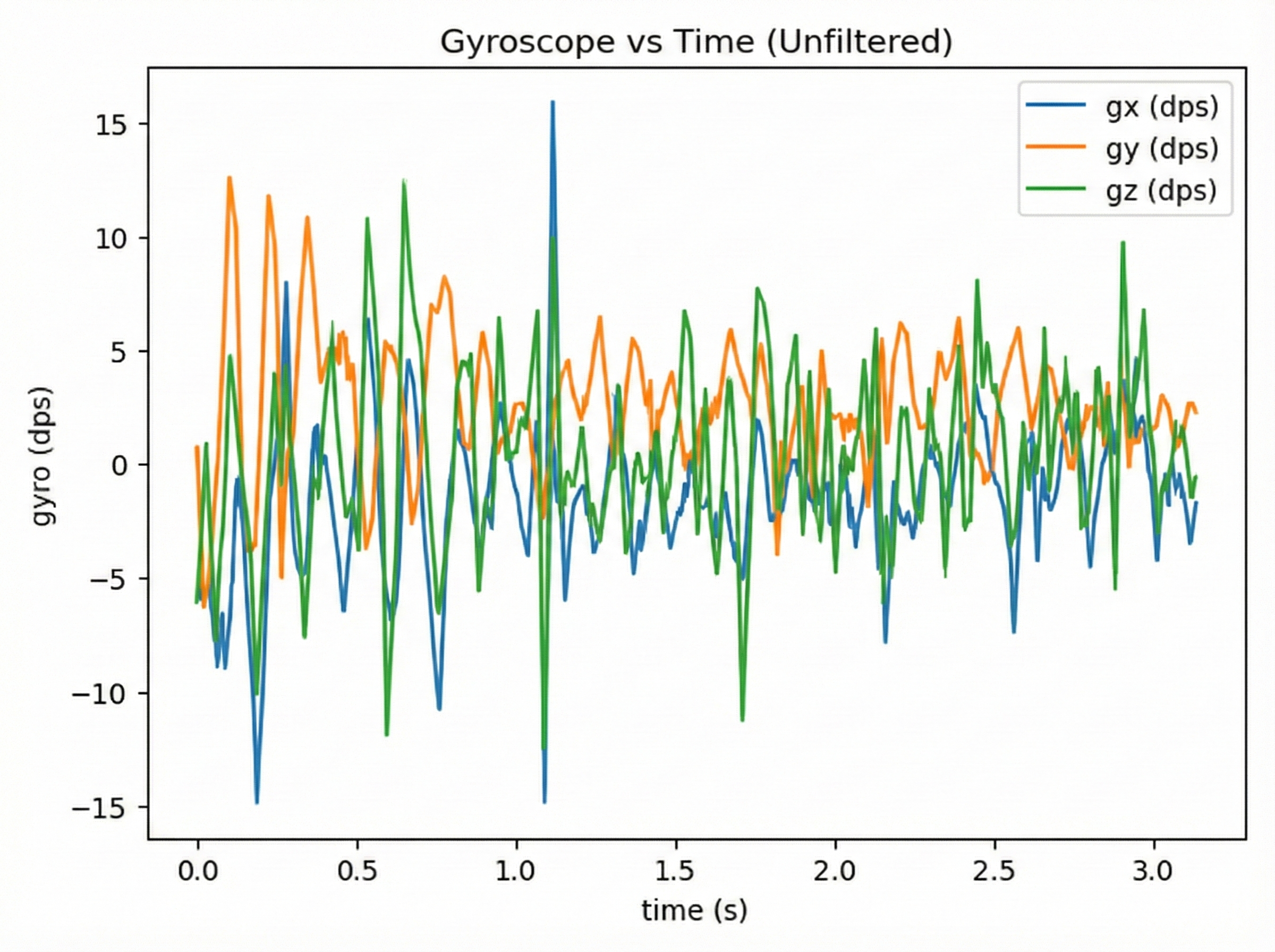
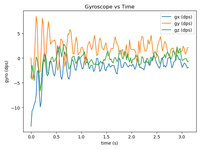
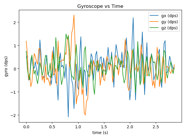
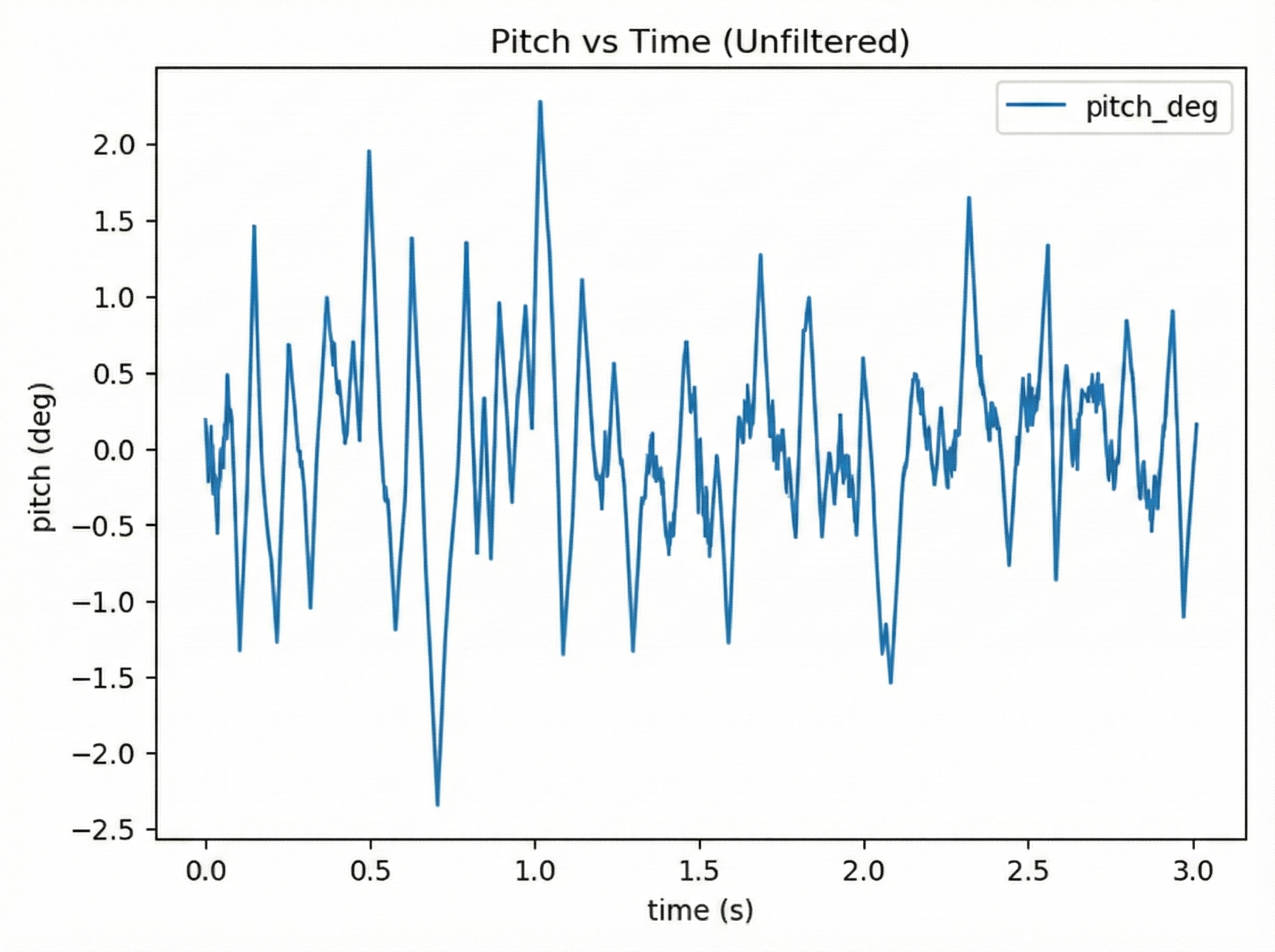
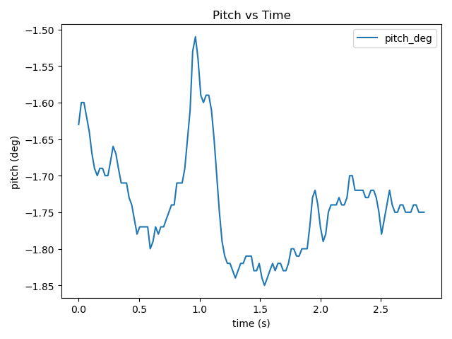
In static pitch experiments, all three filtering methods exhibit varying degrees of drift, with the offset direction trending toward negative values. The unfiltered data near the zero point suggests that data noise dominates the drift effect, making the drift less noticeable. In gyro experiments, unlike the other two groups, the CF’s xyz-axis data showed closer alignment. At system startup, the y-axis rotational angular velocity initially exceeded those of the other two axes, gradually stabilizing near zero. This phenomenon likely stems from the system’s high acceleration during initial operation. CF’s over-correction mechanism may generate excessive torque in the motor, causing the y-axis angular velocity to spike momentarily (also, it could simply be an outlier). The unusually small x-axis value at t=0 is likely an outlier, possibly due to uneven surfaces on the experimental table or other factors that induced a sharp roll angle change.
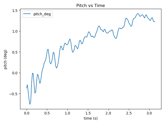
2.Slow Motion
-Pitch


-Gyro


In the pitch angle experiment for slow motion, The introduction of motion makes the data change more violently. Under normal conditions, the unfiltered pitch angle should theoretically have a larger oscillation amplitude than the CF. However, in this experiment, the two values were nearly identical (the unfiltered one was slightly 20% higher), which may be due to the inherent limitations of the MPU6050.
3.Forward
-Pitch


-Gyro

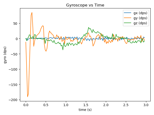
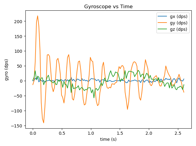
The CF graph from the gyro experiment vividly illustrates the issues caused by CF. When the robot accelerates horizontally, CF’s excessive error correction causes oscillatory overshoots, which is reflected in the graph as the angular velocity on the y-axis fluctuating periodically with a direction that significantly exceeds the values of the other two axes. Generally, the y-axis data shows more obvious changes compared to the other two axes. This is because the robot’s tilting is most noticeable during movement. The second most significant change is the yaw angle on the z-axis, which may result from the robot’s turning due to an uneven table surface.
Overall analysis:
To analyze the performance of unfiltered data, the Complementary Filter (CF), and the Adaptive Complementary Filter (ACF), three metrics are introduced: noise level (jitter), amplitude, and drift. It can be observed that from left to right, amplitude of oscillation decreases.
The unfiltered signal is highly unstable and jagged, which is primarily caused by the high-frequency vibration of the accelerometer and the random walk of the gyroscope. Also the intrinsic properties of MPU6050 is a key factor, since this IMU model is a cost-effective one and may not be ideally stable.
The CF algorithm suppresses this noise by fusing the low-frequency stability of the accelerometer with the high-frequency response of the gyroscope. However, it may still show slight overshoots or lags during rapid motion if the parameters are not optimized.
In contrast, the ACF further optimizes performance by dynamically adjusting the gain based on external acceleration. This method effectively reduces external disturbances, leading to a trajectory that is sharper and more accurate.
- Code for ACF(Run on Arduino IDE)
https://gitlab.oit.duke.edu/jz532/experimentdesignproject/-/blob/main/ACF.cpp
- Future Work
Although the robot using ACF is significantly more stable than the one using CF, it eventually falls down after a period of slight oscillation. This indicates that while ACF effectively suppresses noise, it cannot withstand continuous external disturbances.
The main reason is that he only applied a Proportional (P) controller to the DC motors. Without derivative action to dampen the overshoot, the robot fails to recover from severe oscillations caused by huge center-of-mass shifts. To achieve continuous self-balancing in the future, PID or PD control is a basic requirement. Several potential approaches can be implemented:
1.Encoder wheel

It consists of a slotted plastic disc (usually 20 or 40 slots) attached to the motor’s output shaft and a photo-interrupter sensor. As the wheel spins, the disc blocks and passes the light beam. The sensor outputs a digital pulse (0 or 1) for each slot passed. For hardware, the sensor on the chassis needs to be mounted on the disc on the wheel, connecting the sensor’s signal pin to an Arduino External interrupt pin. Speed is calculated by:
Pulse Count / Slots per Revolution * Time
This approach is intuitive and low-cost while it cannot tell the direction and its resolution is relatively low. A 20-slot disc means 18° rotation per pulse, which leads to oscillation.
2.Encoder motor
It integrates a magnetic Hall effect sensor and a magnetic disc on the rear shaft of the motor (before the gearbox). As the motor spins, the sensor detects the changing magnetic field and outputs two square wave signals (Phase A and Phase B) with a 90-degree phase shift. The motor has 6 wires (2 for power, 4 for the encoder). Connect Phase A and B to the microcontroller’s interrupt pins.
Total Pulses per Revolution = Encoder PPR * Gear Ratio
It has very high resolution and precise direction, even when the speed is low it provides good feeback, but the drawbacks are relatively high cost and complexity because it has more pins so for hardware and software there’s going to be extra works. With more advanced MCU and encoder motor, we can also try more complex control and filter algorithms, like LQR and Kalman Filter.[2]
ME Design Overview
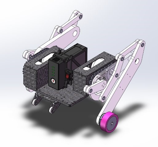

The robot is mainly divided into two modules: the chassis and the legs. For the chassis, we have simplified it and used a 3mm Al plate as the main body, which can carry the battery and the motor base. The robot’s leg module consists of a meticulously designed dual-motor coaxial output module and an open-chain five-bar linkage. All designs were first subjected to finite element analysis in SolidWorks to ensure that the mechanical strength met the required safety factor of 2.0. Then, we used 3D printing to create prototypes to ensure that they conformed to the assembly sequence and eliminated all mechanical interferences. Finally, we used CNC machining to process the leg parts.
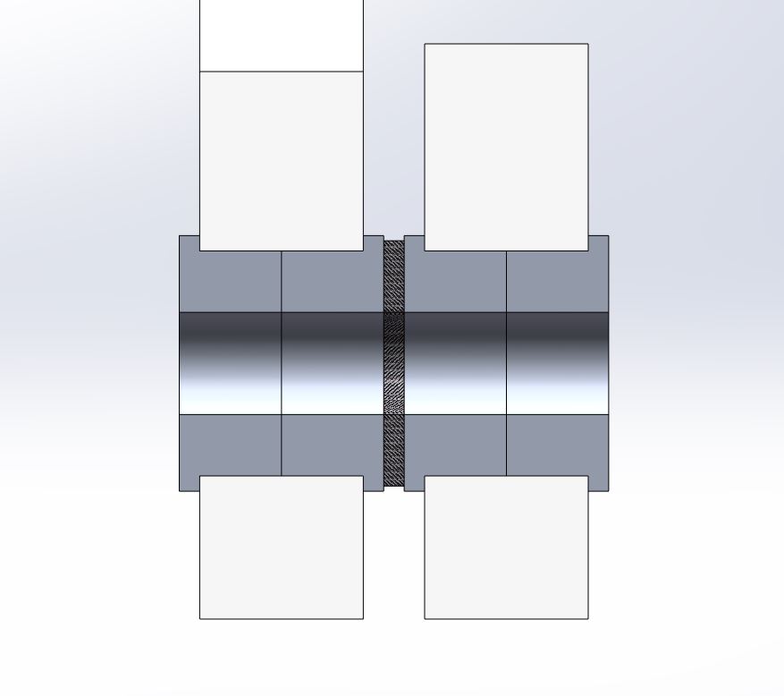
Coaxial Output Shaft Design:

To drive the open-chain five-bar linkage, we designed a coaxial dual-motor output module. In the diagram, the red section corresponds to Motor 1, which actuates the front-thigh linkage, while the green section corresponds to Motor 2, which actuates the rear-thigh linkage. To maintain coaxial alignment for Motor 2’s output, we implemented a chain-drive transmission, which also helps minimize step loss. For smooth and independent rotation of both linkages, needle-roller bearings are used to decouple the two mechanisms. Additionally, to prevent axial shift of the front-thigh output shaft, we incorporated thin-walled deep-groove ball bearings, providing support and reducing bending displacement at the distal end.
The assembly process for this mechanism is also quite specific. Starting with the red component and the output shaft of Motor 1: the first red output flange (on the left) is directly bolted to the motor, with four M3 hex nuts pre-positioned inside before fastening. After that, the needle-roller bearing is installed over it. For the green component, the sprocket flange and the rear-thigh link are connected using six M3 countersunk bolts. Two ball bearings and the red No. 2 extension spacer are then inserted into the inner portion of this subassembly. Finally, the front-thigh output shaft serves as the end cap, and four M3 × 40 bolts are used to engage the pre-placed nuts in the first red output flange, completing the assembly.
Open-chain five-bar linkage Design:
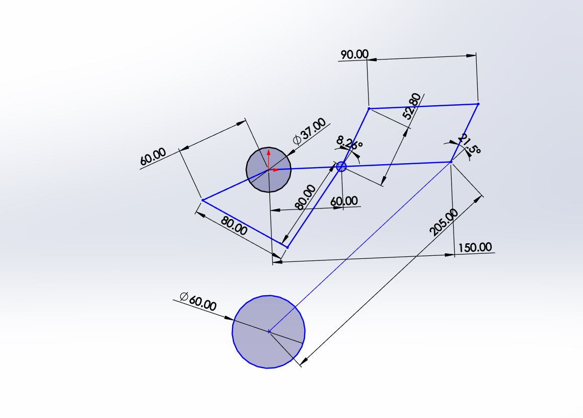
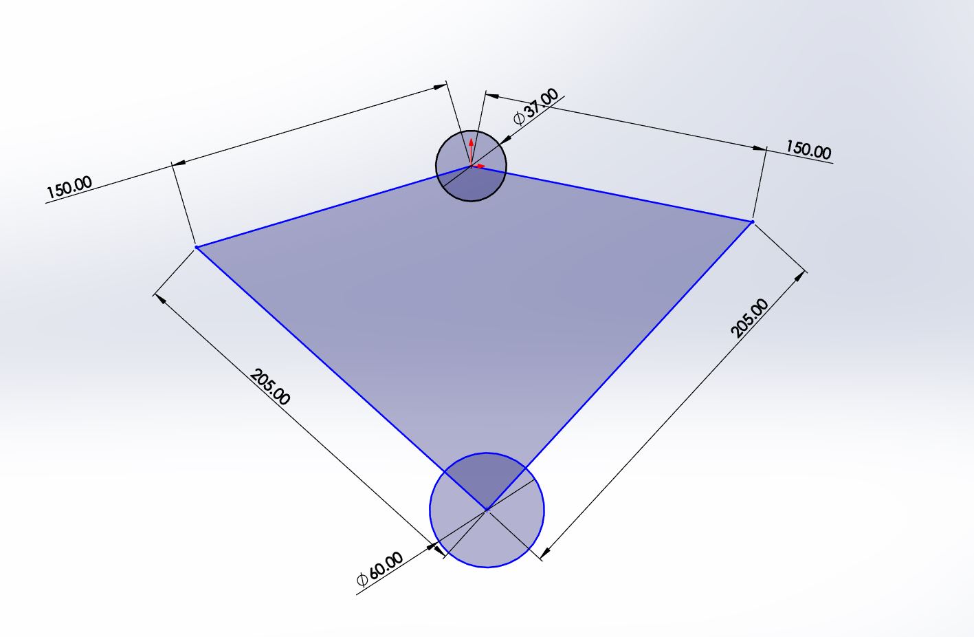
The Linkage parameter:
For the design of the open-chain five-link linkage, the first thing to define is the length of the thigh and calf. Here, we refer to the parameters from the Tencent Robotics article and scale them down by half. Another key design consideration was how to effectively replace the front calf link. We used SolidWorks sketch functions to redraw the linkage sketch, and we successfully got the equivalent mechanism by adding two linkages parallel to the rear thigh and calf.
Linkage joint:
To ensure smooth operation of the entire leg-pivot mechanism, we used plug screws and flange bearings to form each shaft system, and added shims to prevent lateral bending of the links. For the screw–bearing interfaces, we designed a −0.1 mm allowance in the 3D-printed components to achieve an interference fit, allowing the bearing to seat firmly without introducing excessive play. For the final machined metal parts, we specified a +0.01 mm tolerance to achieve an appropriate clearance fit. During discussions with the workshop technicians, we also learned an additional practical technique: creating three or four small center-punch indentations inside the shaft bore. These indentations act like clamping tabs that securely grip the bearing. In practice, this method proved to be highly effective.
Jacobian Matrix of Traditional 5-bar linkage:
age: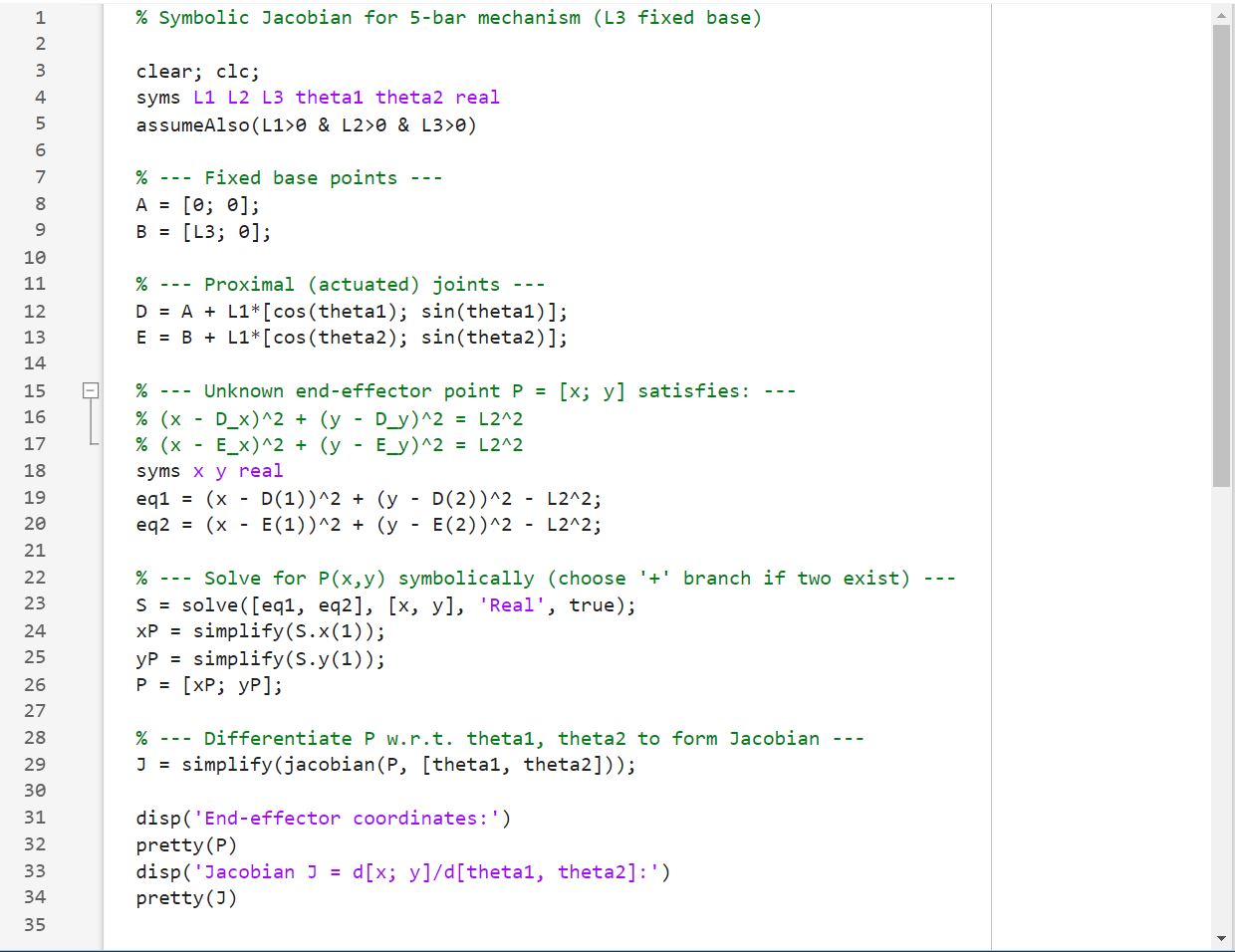
For our design, L1 = 0.15, L2 = 0.205 L3 =0. Then we have the result below with theta1 = 15 deg, theta2 = 165 deg (trial). As shown below, the MATLAB result agrees with the SolidWorks sketch, so the Jacobian Matrix is correct.


Simulation:
In the simulation section, we begin with a comprehensive mechanical analysis of the robot as an integrated system and derive the corresponding state-space representation and control input vector for LQR controller design. The resulting model is then implemented in MATLAB/Simulink, where a multibody dynamic model is constructed to perform motion simulation and evaluate the controller’s performance within a simulated environment.
System Modeling
For the robot’s balance and longitudinal motion problem, the focus is mainly on the posture of the robot’s upper mechanism and legs, as well as the motion of the drive wheels. The change in leg length is ignored; only the leg posture is considered, i.e., the angle of the line connecting the drive wheel axle and the center of the two leg joint motor axes relative to the inertial frame. The robot’s upper mechanism is called the body(chassis), and the line connecting the drive wheel axle and the leg mechanism’s axis of rotation is called the pendulum, resulting in the wheel-leg inverted pendulum model shown in the figure.

![]()
After using Newton and Euler method to analyze the torque and the force on wheel and body, we finally get this state vector and control vector.
What is LQR?
Linear Quadratic Regulator (LQR) is a model-based, state-feedback control method designed for linearized dynamic systems. It computes the control input by minimizing a quadratic cost function that penalizes both state deviations and control effort, resulting in an optimal feedback law that stabilizes the system while balancing performance and actuator usage. Because the control input is calculated using the full system state, LQR naturally accounts for the dynamic coupling between multiple states and inputs.


Why LQR?
Compared with PID control, LQR is better suited for wheel-leg balancing robots, which are inherently unstable and strongly coupled systems similar to an inverted pendulum. PID controllers operate on individual error signals and are typically tuned in a single-input–single-output manner, making it difficult to systematically handle interactions between wheel motion, leg dynamics, and body attitude. LQR, by contrast, treats the system as a multivariable whole and optimally coordinates wheel and leg torques to maintain balance.
MATLAB Simulation
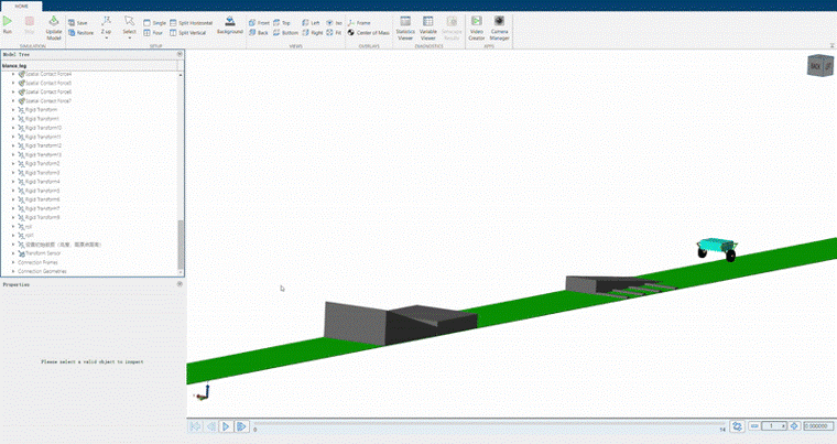
The simulation environment setup is as follows: First, the robot is dropped from a height of 0.2 m, then passes through an asymmetrical 5 deg slope and a bumpy road to test its roll angle balance. After that, it jumps onto a 0.2m platform and overcocme a 10 deg slope. The entire process takes around 20 seconds.

Manufacturing Process
The primary part that requires manufacturing is both legs of out wheel-leg bipedal robot. In the first place we made a 3D printed model to verify our mechanical system stability and if there are any structural conflict within our chassis and legs. With our prototype functioning properly, we then moved on to our manufacturing stage. For our robot, calf, thigh and multiple calf linkages are required to be manufactured, and the positions and diameters of holes require precision to 0.0001. The manufacturing material we picked is aluminum, and the reason why we did this is that picked is good in terms of strength and also adds appropriate weight to our entire robot. And when it comes to our manufacturing processes, aluminum is easier to cut compared to stainless steel and it has way less health impair possibilities.
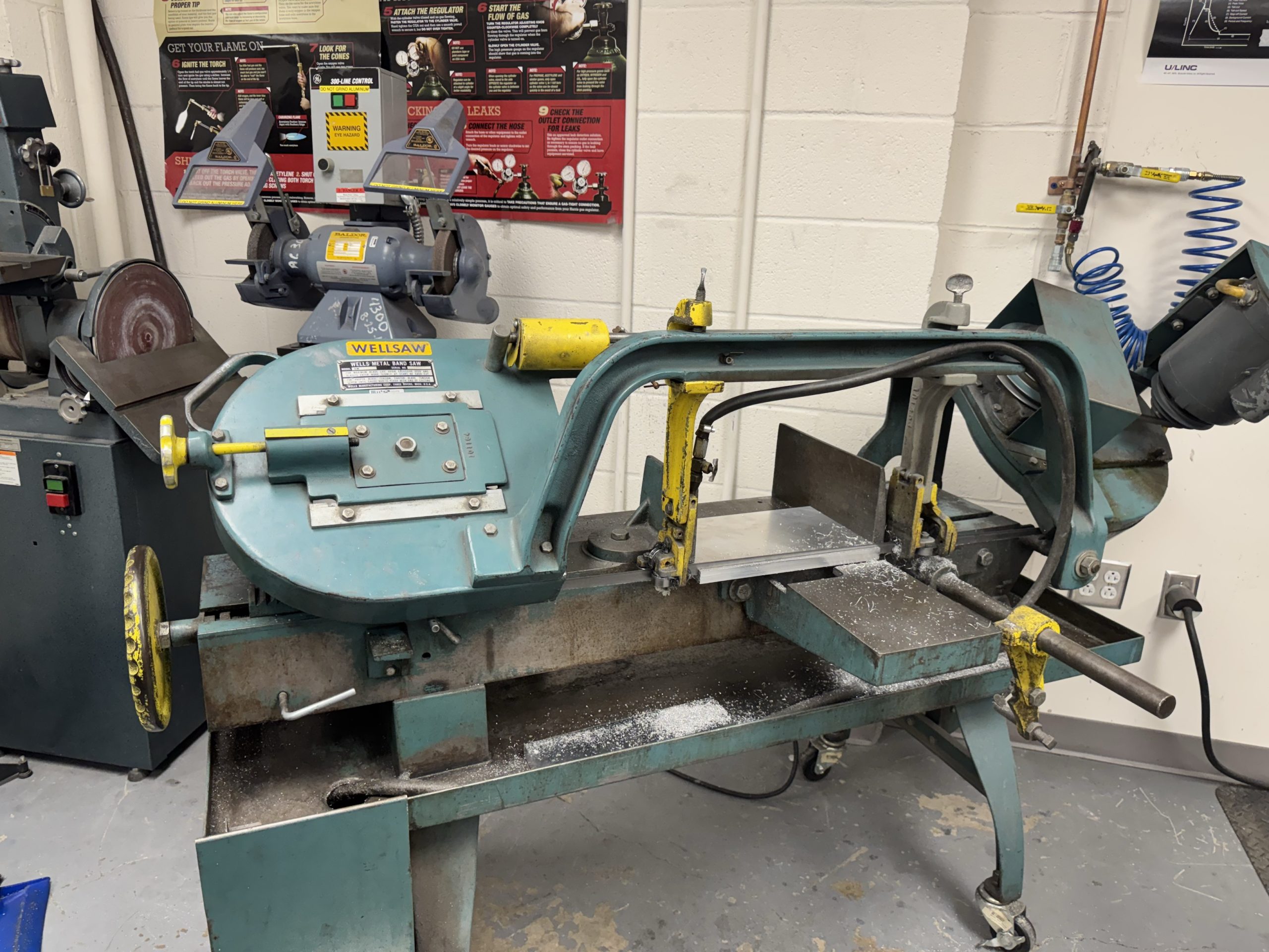
The entire manufacturing spans about a month and a half, and I’m mainly in charge of the whole process and Ray was helping along the way. With our CAD design at hand, we placed our order of 3 aluminum plates and thought through what our manufacturing processes are and what tools and machines are going to be utilized to maximize our precision and efficiency. And here’s the machines we picked and why:
Mill: The primary function of mill is removing material from stock and flattening and smoothening surfaces. Also, mill can be used to cut slots and keyways, drill, bore and tap. Advanced CNC milling machines can also be used to create 3D surfaces and do automatic machining.
Lathe: Lathe is a bit different in terms of rotating pattern. Lathe would rotate the material instead of the drill bit and push the material against the cutting tool to achieve machining purposes. Normally lathe would be used to cut cylindrical and conical shapes. Instead of plates and cubes, lathes would be used for rods, shafts and some other round materials.
Band Saw: Band Saw is a very efficient but coarse cutting tool. The band runs on two or more wheels, which rotate continuously to move the blade in one direction, allowing for smooth and consistent cutting. But normally under circumstances like precision cutting, mills would be required to cut to the exact size.
Arbor Press: Arbor Press is a manual machine to apply forces to press for assembly and other tasks. The main function is pressing bearing into housings, broaching keyways and bending materials


On top of these professional machines, some other hand tools are used as well. Hand drills are used to cut positions that don’t require precision and, in the meantime, save time. For example, when we’re deburring newly drilled holes and holes that aren’t required to edge find, hand drills will be used to improve efficiency as it’s normal to spend days on one piece of metal.
The first metal piece we cut is the calf link. The manufacturing processes entail drilling two holes, clearing out a central slot and milling them down to proper size. Counterintuitively, even though this is the smallest piece we have, and it’s way smaller than the other two pieces we have cut, it took us longer than a week to finish it. One reason is that we were still at the stage of finding the best way to finish the manufacturing processes, the other one is that this linkage needs to be super precise and when we were milling it down with the end mill, we could only remove the aluminum bit by bit and making two exact pieces is quite time consuming.

The second part and the third part are somewhat similar. The manufacturing processes are cutting them down to approximately the size and shape we’re looking for, edge finding and drilling the holes and remill them all down to the exact size. One big addition to our manufacturing this time is introducing MDI and G-Code. Our thighs and calves are gnarly looking and it’s almost impossible to cut out the shape manually. And also one hole on our thighs exceeds the biggest diameter we have off of our drill bits, so we were forced to introduce MDI and utilize reamers to achieve the diameter we’re looking for.

This semester, we primarily completed Steps 1 and 2 of the project. Some time was unavoidably spent on motor selection and CAN bus implementation, as the ESP32 did not perform as reliably as expected for CAN communication. As a result, we transitioned to a USB-to-CAN converter for more stable operation. Despite these challenges, we successfully validated the feasibility of both the mechanical design and the control algorithm. We also implemented a simplified inverted-pendulum-cart demo to verify the robot’s balancing capability, also the stand-up function and leg-length control on the test bench. Overall, this work has established a solid foundation for future development.
Open-Chain five-bar linkage Wheel-legged Robot test bench

 Wenkang Li
 Junyan Zhou