

Motivation
With the ever-increasing complexity of engineered materials, it is more critical than ever to decrease barriers between the fabrication of experimental designs and formal performance testing. Many of the material testing systems currently utilized in research are large, expensive pieces of equipment that are often far-removed from the makerspaces where materials for testing are designed and fabricated.
In order to expedite the prototyping process, this project aims to create an easily accessible, low-footprint material testing system and test this device using a novel material specimen design pipeline.
Background
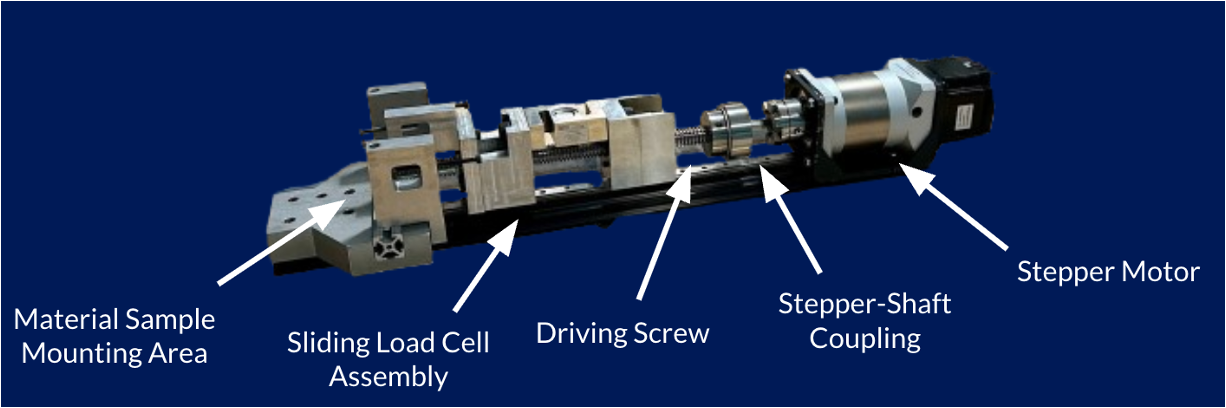
In an attempt to improve materials testing accessibility, a previous Duke project developed an initial prototype for a bench-top materials testing device. This device can be seen below, in a configuration intended to perform bending tests:
Areas for Improvement
While a promising start, this existing design does feature several important areas for improvement. After examination of the quality and convenience of the testing apparatus, the following problem areas were identified:
- Motor Subjected to Axial Force: The coupling linking the motor to the threaded driving shaft was filled with dried epoxy, likely to resist tensile force in the driving screw. As a result, the coupling could not fully engage. While a new coupling is certainly needed, the larger issue to address is preventing axial force from reaching the stepper motor in the first place.
- Inconvenient Test Setup Procedures: The current design requires users to fully disassemble the entire apparatus to transition to a different test. This process is inefficient and difficult. Having one general setup where subcomponents can be swapped and easily moved around for different tests would make for an easier user experience.
- Lack of Robust Physical Interface: There was no way to control the motor outside of the controller’s virtual interface. Having physical controls would allow for use of the machine without the need for a laptop and make for an easier test setup process.
- No Ability to Collect and Analyze Test Data: The current system did not feature a load cell amplifier, meaning users would be unable to interpret the small voltages coming from the load cell during tests. Further, the torque gauge being used had no wired data output, meaning there was no way to collect precise torque data over the course of testing.
- Unorganized Electronics: Controls and wiring were exposed and unorganized on the original system. Having a more formal, polished user experience would make for a safer, more reliable experimental apparatus.
Project Statement
“We aim to expand on the work of previous students to design, fabricate, and test an improved, user-friendly bench-top material fatigue testing system with the goal of optimizing gyroid lattice design through physical testing, finite element analysis, and Bayesian Optimization.”
System Structure
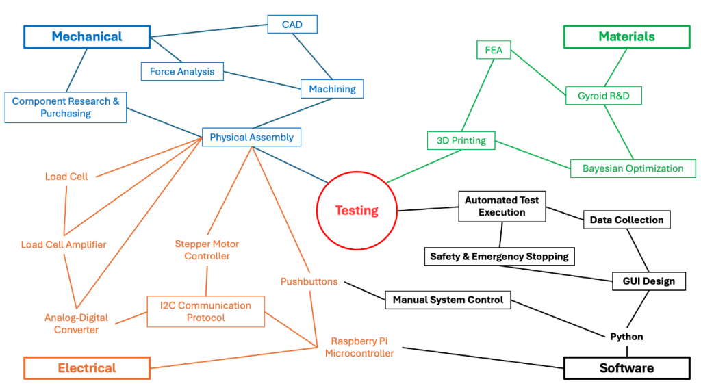
Design Breakdown
Given the many components of this project, we have compartmentalized each critical area of development into separate pages. If you are curious about the material science, mechanical design, electronics, or software development portions of the project, navigate to the relevant subtopic using the navigation buttons below:
Materials Research
Motivation
Lightweight efficient structures are critical in many applications in aerospace, biomedical engineering, automative engineering, and personal safety. They provide a comparable mechanical performance at a fraction of the weight as solid structures. There are many techniques to designing efficient structures. One of which is topology optimization. However, this process is slow and iterative and results in uniquely shaped structure which are difficult to manufacture. Gyroid lattice structures provide easily replicable and manufacturable geometries that are still porous and efficient compared to topology optimization. They still however, are computationally expensive to evaluate. Bayesian optimization will not only allow us to explore the most optimal gyroid designs, but will also enable us to predict the stiffness of any gyroid lattice with a degree of certainty.
Lattice structures have far reaching applications in biomedical, aerospace, and personal safety applications. Their high porosity makes them ideal for surgical implants, maximizing the processes osseointegration [2]. Lattice materials are also being explored for morphing wing skins and other adaptive structures, where their low density and tunable mechanical response directly translate to improved efficiency and performance in weight-critical aerospace systems [1]. In personal safety applications, the ability to crush and absorb energy makes them at the forefront of research in such applications as helmets and bumpers on cars [3].
Gyroid Geometry
The gyroid is a TPMS structure defined by the implicit surface equation below:
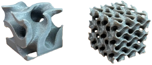
By connecting gyroids together in such a way we can generate lattice structures as seen below.

The gyroids unique topology proved a continuous interconnected material distribution when connected together. This provides a high surface area-to-volume ratio with smooth stress flow paths and minimal stress concentrations [7]. These characteristics make gyroid lattices particularly suitable for additive manufacturing and structural optimization.
Geometry Generation
Three design parameters of Gyroid lattice structures are explore: porosity, periods, and grading. Porosity is defined as the amount of open space in the geometry. A period is one complete unit cell of the repeating pattern, or in other words, how many complete sign curves are in each edge. Grading is spatially varying the material from top to bottom. The bottom of the gyroid lattice will be more dense than the top. This is done to help with shock absorption and crushing of the lattice in many applications. All three of these input parameters effect the efficiency of the geometries. To which extent however is unclear as is the optimal combination of the three.
The geometries are efficiently generated as STL files with controllable design parameters. This allows for easy exploration of the design space. The script simply accepts the design parameters as well as a cube size (25 mm for this study) and generates the STL.
Mesh Generation
To perform FEA, the STL geometry needs to be discretized into a mesh. Meshing such complex structures can be challenging and computationally expensive. Many commercial FEA software packages have built-in mesh generators; however, they are limited and will not work with these complex geometries. Instead, Gmsh, an open-source three-dimensional finite element mesh generator, was used. The STL files were imported directly into the Gmsh workflow to generate volume meshes using tetrahedral elements, which handle complex geometries effectively. A mesh convergence study was performed to ensure the mesh density provided sufficient solution accuracy.
Finite Element Analysis
Once a mesh is generated, the structure is ready for finite element analysis. FEA simulation were done in MOOSE, a massively parallel finite element simulation framework developed at Idaho National Laboratory. The material model used is representative of PLA (E=3000 MPa, Poisson’s ratio=0.6) and assumed to be Linear Elastic. The sample was fixed on the bottom edge in all directions, and a displacement BC was applied in the negative Z direction on the top face of the specimen. The total displacement was -0.025 mm or a 0.1% strain. Although small, we wanted to ensure the test stayed applicable to linear elasticity and the PLA would not break (~0.5% strain). The test outputs displacement fields, von-mises stress, forces, and derived quantities such as effective stiffness which will be used as the objective in the Bayesian optimization model.

Bayesian Optimization
To explore the design space, we employ Bayesian optimization, a sequential model-based optimization approach well-suited for expensive black-box functions like finite element simulations. This method provides a principled framework to direct the search in a way that is both explorative and exploitative: it explores uncertain regions of the design space while simultaneously exploiting promising areas to converge toward optimal designs.
Bayesian Optimization works by building a probabilistic model of the objective function called the surrogate model. This is usually assumed to be a Gaussian Process (GP). The GP provides both a mean prediction and uncertainty estimate at any point in the design space, the GP is continuously updated as simulations are performed. It can be written as:

where m(x) is the mean function (often assumed to be zero) and k(x, x’) is the covariance kernel function, which is chosen to be the radial basis function (RBF) kernel. At each iteration, the GP provides both a posterior mean μ(x), representing the predicted objective value, and a posterior variance σ²(x), quantifying the uncertainty in that prediction. These are then used by an acquisition function to select the next design to evaluate.
The other key piece of Bayesian optimization is the acquisition function. This function will actually look at the surrogate model and decide where to sample next, balancing exploration and exploitation. There are many choices for the acquisition function, for this model, Expected Improvement (EI) is used. More specifically, the log Expected Improvement function.
where f(x) is the objective value at candidate point x and f* is the best value observed from previous simulations. EI measures the expected improvement over the current best, balancing the predicted performance (mean) and uncertainty (variance) at each candidate location. The point that maximizes EI is selected for the next FEA simulation. The Log Expected Improvement simply takes the log of the above function to improve numerical stability as the EI becomes small.
Design Workflow
Before the Bayesian optimization could be run we needed to generate an initial dataset. To do this a sample generation pipeline was built which can be seen below:

Latin Hypercube sampling was used to ensure solid coverage of the design space when generating samples. Those inputs were then passed to the FEA pipeline which makes an STL file with the given inputs, builds a mesh from the STL and passes it into MOOSE to be run. The results are output to a CSV and the process is repeated. In total, 261 usable samples were made from 400 FEA sweeps. Some inputs were invalid and could not be meshed. These inputs are handled accordingly via a constraint objective in the Bayesian optimization algorithm. In total, 400 sweeps took four days to complete.
Once the dataset was complete, the Bayesian optimization model was ready to be run. The work flow for the pipeline is shown below:

The surrogate model is recalculated after each iteration, and new sample is chosen for FEA simulation with the acquisition function. This process was run 30 times, resulting in 29 usable samples and taking one day. The one non-usable sample had inputs which could not be meshed properly. Results like these are penalized in the model so the acquisition function knows to stay away from them. In order to ensure a good balance between exploration and exploitation, every 5 samples the model randomly generates a sample, furthermore 1% noise was added to the surrogate model to ensure proper exploration of the design space.
Results
Once the BO was run, the results can be shown in the plots below.

This histogram compares the specific stiffness values achieved by the initial Latin Hypercube Sampling (Global, blue) versus the Bayesian optimization iterations (BO, red). The Global sampling provides broad exploration across the design space, with stiffness values ranging from approximately 900 to 1800 MPa/(g/cm³) and following a roughly normal distribution centered around 1300-1400. In contrast, the Bayesian optimization samples are heavily concentrated in the high-performance region (2000-2100 MPa/(g/cm³)), demonstrating the algorithm’s ability to efficiently identify and exploit promising areas of the design space. This targeted sampling validates the exploration-exploitation balance of the acquisition function.

This three-panel plot reveals how each geometric parameter influences specific stiffness:
Porosity-Stiffness Trade-off: The strongest correlation emerged between porosity and specific stiffness, with lower porosity designs (40-50%) consistently achieving specific stiffness values above 1600 MPa/(g/cm³). The BO algorithm exploited this trend, targeting the low-porosity regime while maintaining diversity across the grading and period parameters.
Grading Effects: The grading parameter shows weak correlation with specific stiffness, exhibiting significant scatter across the design space. This suggests grading has minimal influence on the objective function compared to other parameters.
Period Effects: Period emerged as a critical design parameter, with higher period values (6-8) achieving significantly greater specific stiffness than lower periods (1-3). The vertical banding pattern clearly shows that periods 6-8 consistently reach 1800+ MPa/(g/cm³), while periods 1-3 plateau below 1400 MPa/(g/cm³).
Using the Model as a Predictive Tool
Now that the optimization is complete, the trained surrogate model can be used as a predictive tool for gyroid lattice performance. With 261 random samples and 29 guided BO examples, the surrogate has a great understanding of the design space and can make accurate predictions across it. This predictions can be made rapidly, compared to waiting 30 to 40 minutes for the finite element simulation to run.
A prediction script was developed that accepts three input parameters (porosity, grading, period) and returns both the predicted specific stiffness and associated uncertainty (confidence interval).

The script will then ask the user if they’d like to verify this result with an FEA simulation. If the user says yes, then the script will automatically run the simulation in MOOSE and then compare the simulated result with the predicted result and give the percent error.

This enables rapid design space exploration and what-if analysis without the computational expense of finite element simulations.
Mechanical Design

Objectives
- Resolve existing design flaws
- Increase structural rigidity
- Design multi-purpose elements that can be used across testing modes
Preventing Axial Force Transmission to Stepper Motor
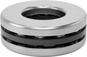
In order to allow a driving screw to rotate freely without transmitting axial force back to its driving motor, a thrust bearing is commonly used. Composed of two washers and a central ball-bearing assembly, a thrust bearing sits between a rigid structure and a threaded, locking shaft collar. Axial force is transmitted from the shaft to the shaft collar, to the thrust bearing, and into the rigid structure, allowing the driving motor to remain in purely torsional operation.

Using the two components above, the following component was designed to absorb all compressive axial force in the driving screw.

Positioned just in front of the motor-coupling assembly, the axial force absorber (colored green above) protects the stepper motor from any compressive loading.
Improving Structural Rigidity
To channel load paths through metal structural elements versus an acrylic panel, the T-slotted base rail for the machine was mounted directly to the bottom of the surrounding protective cage using added cross-bracing.

In addition to the cross bracing, a larger triple T-slot base rail was purchased to more easily integrate with the cross bracing while also providing more support.
Finally, more durable linear sliding carts were used in combination with a stronger sliding rail to increase structural rigidity while still allowing fluid, low-friction motion of the two sliding elements of the machine, the threaded and non-threaded load cell mounts.

Designing Multi-Purpose Machine Elements
In order to minimize the overall number of machine components needed and expedite the transition between testing modes, a major redesign of the machine was conducted to ensure material efficiency and ease of use. Shown below are the four testing modes with identical components marked with the same color.
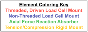
As shown above, the compression and tension assemblies were designed with exactly the same components, but in a flipped orientation and with a different driving screw nut. The bending assembly mimics the compression assembly, but with a different specimen contact attachment and end brace assembly.
Static Analysis
To evaluate the structural integrity of the proposed designs, two specific areas were investigated: the nominal limits of the linear sliding carts and the bolted connections keeping components together. Each area was evaluated to determine whether the maximum 500 kgf (1100 lb) rating for the load cell could be achieved by the machine, or if not, what the greatest loading could be.
Linear Sliding Cart Analysis
Based on the documentation for a HGH20CA slider, the model can withstand 200 Nm about Mp, as shown below.

Mp is the only moment axis directly relevant to the proposed designs, so static analysis was performed to determine the maximum allowed loading for the machine as it relates to this failure mode. Two of these carts are used in the design, one below the threaded load cell mount and one below the non-threaded load cell mount. The cart beneath the threaded load cell mount would fail prior to the cart beneath the non-threaded load cell mount based on the way force is applied to each component.
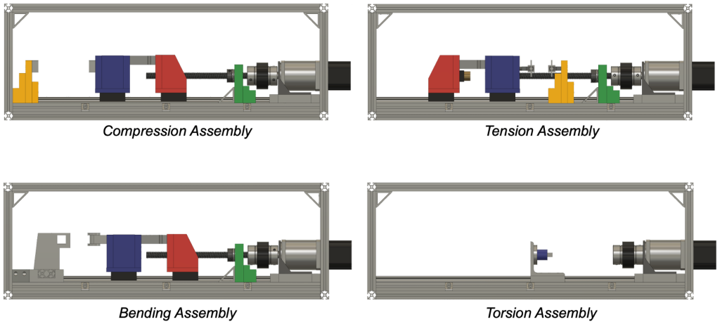
As shown below, we see that the larger moment arm (1.825in or 0.046355m) created in the red, threaded load cell mount would result in a larger moment reaction Mc1 compared to Mc2.
Thus, if we only consider Mc1 and set F equivalent to the 500 kgf (4903 N) maximum rated force for the load cell, we obtain an Mc1 equivalent to 4903 N * 0.046355 m = 227.3 Nm, exceeding the maximum moment rating for the cart. Therefore, the maximum allowed force, as measured by the load cell, must be less than or equal to 4314 N, or around 970 lb.
Bolted Connection Analysis
We performed similar analysis to determine the whether bolted connections would result in an even smaller maximum allowed force. Across all designed components a minimum of 10-24 alloy steel bolts are used. Each of these bolts is rated for 170,000 psi, with a tensile stress area of 0.017 in^2, so each bolt is able to withstand up to 2890 lb. Since the load cell rating limits the device to an 1100 lb maximum load, we see that even a single bolt could withstand the maximum load for our device. With this in mind, we attempted to examine the various moments created in our components to see if any larger forces were observed.

Starting with the axial force absorber, we see that if we assume the corner brackets are missing, and 1100 lb is applied through the shaft, a bolt response moment of 1303.5 in*lb is necessary to withstand this load.
With 4 bolts contributing to the response moment, and 4 total bolts securing the component to the base rail (ignoring the corner brackets), the force absorber is certainly not limiting the maximum allowed force for the machine.

With 4 bolts resisting an even smaller moment in the case of the tension/compression end brace, this component does not seem to limit the allowed maximum force lower than linear cart analysis.

Alternatively, if we assume that only the bolts in the front plate of the end brace can resist the moment create about the bottom of the brace, we are left with 2 1/4″-20 bolts needing to withstand a 4730 in*lb moment. With the bolts being 2.5″ from the pivot, we see that the the combined bolts would need to withstand 1892 lb, or 946 lb each. This is no issue as these bolts, with tensile stress area of 0.031 in^2, can withstand 5270 lb each.

Finally, as a last check for the the bolts subjected to the most load, we took a look as the threaded load cell mount, specifically its bolts connecting the aluminum to the cart. Under max load, there is a 4180 in*lb moment about the bottom right corner which must be countered by 4 M5 bolts. With a tensile stress area of 14.2 mm^2 (0.022 in^2), each alloy steel M5 bolt is rated for 3740 lb, plenty to withstand this load.
Static Analysis Conclusion
After performing static analysis involving both the linear sliders and various bolted connections, we see that the linear sliders are the limiting variable for maximum loading. With the current linear sliders, we must limit force to 970 lb, barring any further limitations from other project systems.
Fabrication
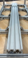
Given the extensive time needed to fabricate all of the necessary components above, the choice was made to focus solely on fabricating the components necessary for the compression and tension assemblies, as these two testing modes consist of identical elements. The machining process for all components followed the progression below:
Step 1: Plan cuts on raw aluminum.

Step 2: Rough cut all elements to shape.

Step 3: Square the sides of each component by milling two opposite sides parallel to each other, and milling the remaining two sides perpendicular to the first two.
Step 4: Mill components down to design-specified outer dimensions.

Step 5: Mill any fine details.

Step 6: Drill and tap holes for securing components to each other or attaching to base rail.

Step 7: Assemble completed components
Threaded, Driven Load Cell Mount
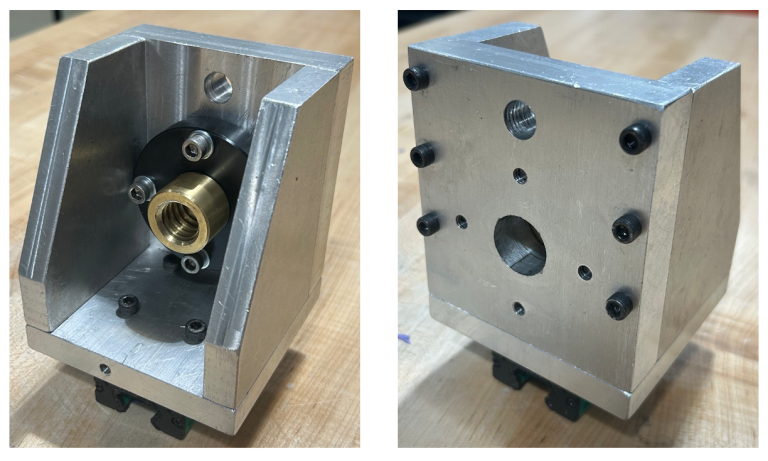
The threaded load cell mount is the component the transfers the rotational motion of the driving screw into linear force. This linear force is transmitted into the load cell, which is mounted using the unused mounting hole visible in the images above.
Non-Threaded, Non-Driven Load Cell Mount
The non-threaded load cell mount supports the other side of the load cell and transfers the force from the load cell into the material specimen. This component integrates with various material contacts for the various testing modes: compression (flat plates), tension (grippers), and bending (rounded protrusion).
Tension/Compression End Brace

The tension/compression end brace supports one end of the material specimen. This component rigidly withstands all the force applied to the specimen.
Axial Force Absorber

The axial force absorber integrates with a thrust bearing assembly to prevent axial load from reaching the stepper motor. This component also acts to support part of the vertical weight of the shaft to maintain alignment.
One thrust bearing washer was press fit into the force absorber using a hydraulic press after milling a mounting hole a few thousands of an inch smaller than the diameter of the bearing washer. This ensures one bearing washer is firmly rigid while the other is free to rotate.

Motor Mount

The motor mount integrates the existing steel motor support bracket with the new T-slot base rail and also adjusts driving screw height in response to the taller linear rail sliders.
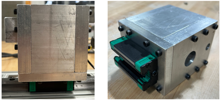
Full Design Overview
After fabrication, we were able to successfully assemble the newly-purchased and created components together with the existing stepper motor and load cell in a more user friendly and robust design.
Electronics & Controls Design

Overview
This project involves the integration of many electrical elements, all essential for controlling the device, gathering data, and creating a pleasant user experience. Here is a brief overview of each component:
Raspberry Pi
As the chosen microcontroller for the system, the Raspberry Pi initiates efforts to control the stepper motor, handles manual controls, parses data from the load cell, operates GUI logic, and gathers experimental data.
Stepper Motor Controller
The stepper motor controller utilizes I2C communication from the Raspberry Pi to translate into motor commands. This device also provides the motor with its operating voltage of 24V. If the controller is plugged into a computer itself, it prompts the user with a GUI to control the motor and modify motor settings.
Load Cell
This 500kg load cell with a 10-15V excitation voltage provides the analog signal needed to understand the load being subjected to a material sample. This device can measure both tensile and compressive force, making it a critical tool for our application.
Load Cell Amplifier
Because the load cell, even at max excitation voltage, still outputs signal on the millivolt scale, in order for these signals to be read, they must be amplified. The chosen load cell amplifier boosts load cell output to a 0-5V range.
ADC Converter
Because the Raspberry Pi is unable to read analog signal, an ADC converter is used to translate amplified load cell signal into the I2C communication protocol, which is able to be read by the Raspberry Pi’s I2C pins.
Pushbuttons
Pushbuttons act as the physical interface for the control of the stepper motor. During setup and transitions between tests, the user can press pushbuttons to rotate the motor and reconfigure the testing setup.
Electrical Limitations
Due to the choice of load cell amplifier, the ADC converter is receiving up to 5V input, which could be transmitted to the Raspberry Pi’s input pins if the ADC converter were to be powered at 5V. Since the Raspberry Pi’s input pins are limited to 3.3V, sending it 5V would damage the pins.
Thus, we are currently powering the ADC converter at 3.3V volts, capping its output to 3.3V , ensuring the Raspberry Pi is protected. However, while the Raspberry Pi is protected from overvoltage, the ADC is not. If the load cell is subjected to high enough force, the amplifier can still emit up to 5V to the ADC converter. Since the ADC converter is powered at 3.3V, this 5V input would damage the converter. Thus, we are unable to utilize the full 0-5V output range of the load cell amplifier, and, as a result, must limit the force on the load cell.
To mathematically determine the maximum allowed force on the load cell before endangering the electronics, we can first calibrate the load cell with a known weight and perform the following calculations:
Unweighted Load Cell Voltage (zero offset) = V0
Weighted Load Cell Voltage (known weight) = Vw
Known Weight = W
Maximum Allowed Voltage = Vmax
Step 1: Obtain force per volt
W / (Vw – V0)
Step 2: Solve for maximum allowed force
W / (Vw – V0) * (Vmax – V0)
Thus, in our case, with
V0 = -0.013464 V
Vw = 0.746 V
W ~ 175 lb
Vmax = 3.3 V
We have Fmax = 763.47 lb, meaning we must physically limit the load cell from experiencing more than this force either by ensuring specimens fail before reaching this load or implementing software logic to stop tests after surpassing a certain force.
This is clearly lower than the 970 lb limit established by static analysis, so our system is currently limited to lower force by electronics, not physical integrity.
Software Development
GUI Overview
In order to operate the fatigue bench and gather data, the user needs to interact with a virtual interface. This virtual interface takes the form of a Python program that controls stepper motor speed by interfacing with the motor controller, collects and parses load cell data, and allows the user to customize testing conditions.
To build a fully operational GUI, the group utilized PySide6, a python library specific for graphical interfaces. We wanted our graphical interface to have the following capabilities:
- Easy test set up for all test types: Tension, Compression, Bending, and Torsion
- Easy selection between monatomic and fatigue testing, along with various testing parameters
- Live logging and plotting of test results
- The ability to easily get results in the form of a .csv.
Test Setup and Termination
In order to conduct materials tests with our system, the user must interact with our virtual GUI. Currently, the user can only click on compression or tension under the loading type, as the physical elements for the other loading types have yet to be fabricated.
Two test modes are currently implemented: monotonic and fatigue. A monotonic test is unidirectional while a fatigue test is cyclical, with motion in both the loading and unloading directions.
For a monotonic test, the user can select a displacement rate and a failure mode. Tests can end either through timer expiration, set displacement amount, material failure, or an emergency condition. Even during timer expiration or displacement termination tests, if a material failure is detected, the test will be automatically terminated. A material failure in a monotonic test is defined as dropping below 70% of the maximum force achieved during the test.
For a fatigue test, the user must select displacement rate, number of cycles, dwell time, and cycle displacement. Similar to monotonic, material failure detection terminates any fatigue test. However, during a fatigue test, a material failure is defined as current peak cycle force dropping below 70% of the maximum peak cycle force achieved during the test thus far.
Automated Test Setup Procedures
Currently, the compression testing mode first conducts an autonomous setup process that slowly brings the jaws together until 5 lb of force is detected, just enough to suspend the material sample between the gripper and maintain a consistent starting condition.
Once setup is complete, the user simply clicks start test to start the test from there.
Emergency Stop
The GUI grants users access to an emergency stop button on any tab of the interface. When clicked, the emergency stop disables all operations. The emergency stop must be cleared to unfreeze the system. Emergency stops can also be triggered autonomously during testing, when a material failure is detected, maximum allowed force is reached, or communication with the motor is interrupted.
If maximum allowed force is encountered during a test (current 740 lb), the system will automatically stop the test and back the motor off until the load cell detects 0 force. After completely unloading, the system will engage an emergency stop.
See the video linked here for an automated e-stop detection demo.
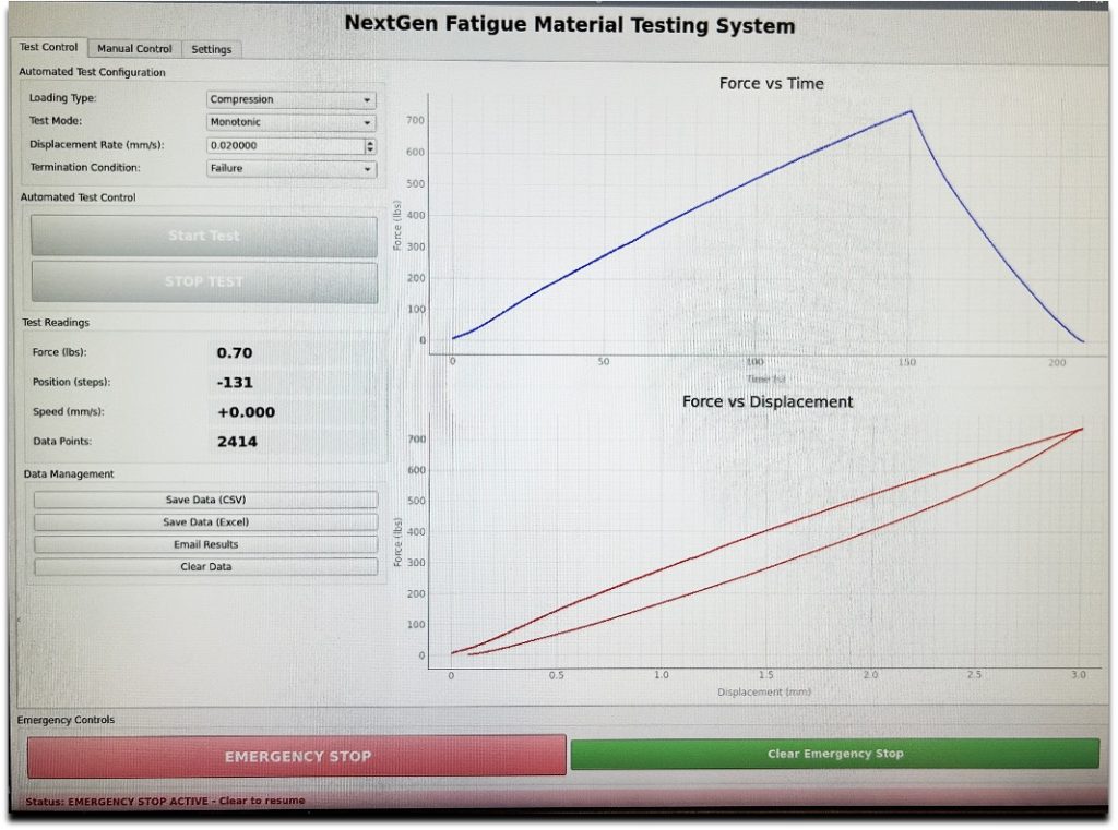
Data Collection and Output
During testing the system automatically collects time, displacement, and force data at 0.1s intervals. Live force vs. time and force vs. displacement plots are shown in the GUI during testing so that the user can monitor the progression of force increase and material deformation during the test.
Upon test completion, the user has the option to export data as a CSV.
Full System Experimental Data
Given that the compression testing mode of the NextGen system is fully operational, preliminary testing data has been gathered. Specifically, testing has consisted of many force cycles up to a maximum of 740 lb with no apparent issues.
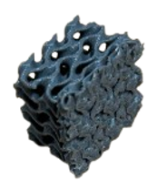
Most interesting, though, is the data collected for a graded gyroid specifically constructed to fail progressively layer by layer. This type of gyroid excels at crushing predictably under load, efficiently distributing impact forces. The force vs. time and force vs. displacement curves for this specimen can be seen below.
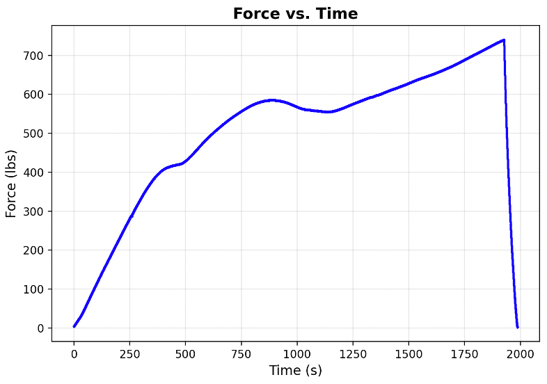
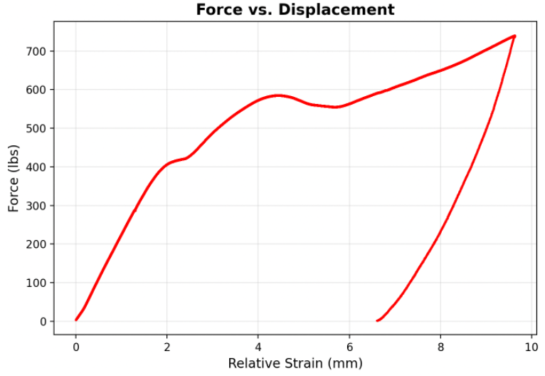
This data fits expected trends, with clear changes in slope indicating transitions from thinner to thicker gyroid layers as the thinner portions slowly crush under large compressive force.
The sharp drop in force and simultaneous reversal in displacement is the automated emergency stop system working as intended. Once the system reached a force of 740 lb, the maximum force currently allowed (minus a small cushion), the motor immediately backs off, reducing force on the load cell until no force is detected.
A before and after image of the tested gyroid can be seen below.

Click here for more raw data collected by the NextGen system!
Future Work
While the NextGen system is operation for the compression testing mode, there are several remaining tasks needing to be performed to support the remaining testing modes.
- Purchase a longer driving screw to support the tensile testing mode. The current driving screw is too short to support the tensile testing mode. An identical 20x4mm type screw will need to be purchased at a size that supports the tensile specimen length.
- Resolve electronic force limitations. Currently, max force is limited by the electronics. The max force could be increased from 760 lb. to 970 lb by using a load cell amplifier that outputs a 3.3V amplified signal range compatible with the ADC converter and Raspberry Pi I2C input limits.
- Finish machining the components for the bending and torsion testing modes. The components for the bending and torsion assemblies have been rough cut but not milled to shape.
- Learn how to use the purchased torque load cell and load cell amplifier. While similar to the load cell currently in use, the torque load cell involves slightly different hardware than the linear load cell.
Links to Project Materials
Video
Check out NextGen in operation here!
Directions for Use
For full directions on how to use the GUI and the testing machine itself, use the QR code below, the matching code on the device itself, or the clickable link below:

User Manual Link
Meet the Team
Click on our photos to check out our personal webpages!


Thanks for Visiting!

References
[1] N. Khan and A. Riccio, “A systematic review of design for additive manufacturing of aerospace lattice structures: Current trends and future directions,” Progress in Aerospace Sciences, vol. 149, 101021, 2024
[2] F. Günther, S. Pilz, F. Hirsch, M. Wagner, M. Kästner, A. Gebert, M. Zimmermann, “Shape optimization of additively manufactured lattices based on triply periodic minimal surfaces,” Additive Manufacturing, vol. 73, 103713, 2023.
[3] M. Kashfi, S.H. Nourbakhsh, A. Amiripour, H.J. Lim, “Constrained functionally graded gyroid structure for tunable energy absorption,” Materials & Design, vol. 258, 114693, 2025.
[4] J. Peloquin, Y. Han, K. Gall, “Printability and mechanical behavior as a function of base material, structure, and a wide range of porosities for polymer lattice structures fabricated by vat-based 3D printing,” Additive Manufacturing, vol. 78, 103892, 2023.
[5] M. J. Uddin, J. Fan, “Machine learning framework to predict the mechanical properties of photopolymer gyroid lattices at various strain rates,” Polymer Testing, vol. 151, 108971, 2025.
[6] Introduction to Bayesian Optimization. Ax Documentation, Meta Platforms, Inc. Available at: https://ax.dev/docs/intro-to-bo/
[7] Peng, X., Huang, Q., Zhang, Y., Zhang, X., Shen, T., Shu, H., & Jin, Z. (2021). Elastic response of anisotropic Gyroid cellular structures under compression: Parametric analysis. Materials & Design, 205, 109706. https://doi.org/10.1016/j.matdes.2021.109706
[8] Zhang, Y., Xue, Z., Chen, L., & Fang, D. (2009). Deformation and failure mechanisms of lattice cylindrical shells under axial loading. International Journal of Mechanical Sciences, 51(3), 213–221. https://doi.org/10.1016/j.ijmecsci.2009.01.006
[9] Zhang, C., Zheng, H., Yang, L., Li, Y., Jin, J., Cao, W., Yan, C., & Shi, Y. (2022). Mechanical responses of sheet-based gyroid-type triply periodic minimal surface lattice structures fabricated using selective laser melting. Materials & Design, 214, 110407. https://doi.org/10.1016/j.matdes.2022.110407
[10] Senhora, F. V., Chi, H., Zhang, Y., Mirabella, L., Tang, T. L. E., & Paulino, G. H. (2022). Machine learning for topology optimization: Physics-based learning through an independent training strategy. Computer Methods in Applied Mechanics and Engineering, 398, 115116. https://doi.org/10.1016/j.cma.2022.115116
[11] Chi, H., Zhang, Y., Tang, T. L. E., Mirabella, L., Dalloro, L., Song, L., & Paulino, G. H. (2021). Universal machine learning for topology optimization. Computer Methods in Applied Mechanics and Engineering, 375, 112739. https://doi.org/10.1016/j.cma.2019.112739
[12] Ruiz de Galarreta, S., Jeffers, J. R. T., & Ghouse, S. (2020). A validated finite element analysis procedure for porous structures. Materials & Design, 189, 108546. https://doi.org/10.1016/j.matdes.2020.108546
[13] Khaderi, S. N., Deshpande, V. S., & Fleck, N. A. (2014). The stiffness and strength of the gyroid lattice. International Journal of Solids and Structures, 51(23–24), 3866–3877. https://doi.org/10.1016/j.ijsolstr.2014.06.024