The Math Behind the SIR Model – The End of the World?

Last updated on April 29, 2020

The SIR model is perhaps the most well known method for simple epidemiological modeling we have today, and as such it is worth understanding how and why it works. This introduction will be for a very basic model that seeks to compute how many people in a given population are susceptible to, infected with, and recovered (or dead) from an infectious disease. For simplicity, we make several assumptions:

1) The population is fixed (those that die from the disease are counted, but neither unrelated deaths nor births are accounted for)
2) Nobody in the population is initially genetically immune to the disease
3) Once recovered from the disease, an individual cannot contract it again
4) The probability of being infected is unrelated to age/gender/race/etc
5) Members of the population mix homogeneously (closed sub-populations that do not interact with outsiders can be individually modeled by their own SIR analysis)

With this all in mind, let us consider some population of $N$ individuals in some spatial space (neighborhood, city, nation, etc) that is subject to some infectious disease. Each person can be organized into one of three groups:

$S$ (susceptible) ~ not yet infected
$I$ (infected) ~ currently infected with the disease
$R$ (removed) ~ recovered from or killed by the disease

If we let $s(t), i(t), r(t) $ denote the total number of people in each of these categories, respectively, which are functions of time $t\geq0$, then the evolution of these functions may be described by a Markov chain: $S \to I \to R$

As we can see, $s(t) + i(t) + r(t) = N$ and the transition flows in one direction only. When a susceptible individual comes into contact with an infected individual, he or she becomes infected with some probability $p\geq\ 0$. On average, at a unit time, an infected individual passes the disease to $p$ susceptible people. Once infected, it takes some random time with mean $1/\mu \in \mathbb{R}^+$ to transition to state $R$. Note that $\mathbb{R}$ is the set of all real numbers, so $x\in\mathbb{R}^+$ means that $x$ is some number in the set of all positive reals.

Now we can use differential equations and the Law of Mass Action to create a proper system of equations describing the rates at which transitions between the states $S$, $I$, and $R$ occur. The basic Law of Mass Action states that the time derivative of the quantity $m(t)$ of some mass equals the difference between the source (causes increase in mass) and the sink (causes decrease in mass). That is, $m'(t) = $ source $-$ sink. Let’s apply this to our model: $S$ obviously has no source, as it is at the beginning of the chain. It has all of the population (or “mass”) before the disease spreads. $S$ can only decrease as people become infected and cannot once again become susceptible. This sink would be proportional to the relative infected population $\frac{i(t)}{N}$ and the infection rate $p$.

$$s'(t) = \frac{-p}{N}i(t)s(t)$$

$I$ has a source from $S$ and a sink to $R$. The source of state $I$ would be equal to the sink of $S$ because people have only one way to exit $S$, and that pathway is the only way to enter $R$. For the sink, $I \to R$ at rate $\mu$, so the sink is given by $\mu i(t)$.

$$i'(t) = \frac{p}{N}i(t)s(t) – \mu i(t)$$

Finally, $R$ has only a source, as it is the last destination anyone can reach, which is equal to the sink of $R$.

$$r'(t) = \mu i(t)$$

We have two notes to make here: First of all, for simplicity we will write any $x(t)$ and $x'(t)$ as just $x$ and $x’$. Secondly, we will make this system dimensionless (so that it does not depend at all on the size of the population) by dividing out $N$. This means that instead of $s + i + r = N$ with $s,i,r$ representing the number of individuals in each category, we have $s + i + r = 1$ with $s,i,r$ representing the proportion of the total population in each category. We therefore have the following system:

$$(s,i,r) = \cases{s’=-psi\cr i’=psi-\mu i\cr r’=\mu i}$$

Readers familiar with basic real analysis might enjoy seeing how we must deal with the question of whether there exists a unique solution to this system. Otherwise, ***feel free to skip over the next paragraph***.

The answer to the above question lies in the generalization of the Picard-Lindelöf theorem for ordinary differential equations in higher dimensions. First of all, the above system, along with the initial condition that $(s,i,r)(0) = (s_0,i_0,r_0) \in \mathbb{R}$, is called the Cauchy Problem (correlated to the SIR model). Let a function $F:\mathbb{R}^d \to \mathbb{R}^d$ be regarded as a vector field on $\mathbb{R}^d$. The ordinary differential equation is given by $x'(t) = F(x(t)), t \in (-T,T), x(0) = x_0 \in \mathbb{R}^d$. A solution $x(t)$ is a function on $(-T,T) \to \mathbb{R}^d$ for some interval $(-T,T) \subset \mathbb{R}$, i.e. a curve on d-dimensional Euclidean space. $F(x(t))$ is the time derivative of the curve, so $x'(t) = lim_{h\rightarrow 0} \frac{x(t+h) – x(t)}{h}$, where the difference in the limit is taken in the sense of vector difference in $\mathbb{R}^d$. $x(t)$ is differentiable at $t$ if the limit above exists and is in $\mathbb{R}^d$. The curve is of class $C^1$ if $x(t)$ is continuous on $(-T,T)$. For $x(t) = (x_1(t),x_2(t),…,x_d(t))$, then $x \in C^1((-T,T);\mathbb{R}^d)$ if and only if each component $x_j \in C^1((-T,T))$. $X$ is a local solution to the Cauchy Problem if it is defined on $(-T,T)$, class $C^1$ on that interval, and satisfies the differential equation above. If $F:\mathbb{R}^d \to \mathbb{R}^d$ is Lipschitz, then for all initial $x_0 \in \mathbb{R}^d$, the Cauchy Problem admits a unique global solution $x:\mathbb{R}^d \to \mathbb{R}^d$. Returning to our $(s,i,r)$ model, set $x(t) = (s(t),i(t),r(t))$, then $x'(t) = F(x(t)) = F(s,i,r) = (-psi,psi-\mu i,\mu i)$ with $x_0 \in \mathbb{R}^3$. There is an issue with the quadratic term $si$, but this is still locally Lipschitz.

***Back to our SIR model***
We are only interested in the case where our initial value (what proportion of the population is in each state at time $0$) $(s(0),i(0),r(0)) = (s_0,i_0,r_0)$ forms a probability distribution. Let’s represent what these values can be in a visual manner. We will use a coordinate system, but instead of $(x,y)$ we will use $(s,i,r)$. Recall that $s+r+i=1$ because the fraction of the population in each state of the system cannot sum to more or less than one hundred percent of the population. This equation forms a plane in 3-dimensional space $\mathbb{R}^3$ which we will call $\Pi$. So any point $(s,i,r)$ must lie on this plane somewhere. So something like $(s,i,r) = (0.2,0.7,0.3)$ would not lie on this plane because $0.2+0.7+0.3$ does not equal $1$. Also recall that $s, i,$ and $r$ must be $\geq 0$, as there cannot be a negative number of people in any category. After all, $(s,i,r) = (-0.2,0.6,0.6)$ has $s,i,r$ adding to $1$ and thus lies on $\Pi$, but has a negative portion of the population susceptible to the disease! Thus, we must only consider the portion of $\Pi$ that is above the $s,i,r$ axes. Let’s call this section of the plane $\Pi^+$. The way we say all of that is

$$(s_0,i_0,r_0) \in \Pi^+ = \{(s,i,r) \in \mathbb{R}^3 | s+i+r=1, s,i,r \geq 0\}$$.

The big blue plane is $\Pi$ and the triangle on that plane is $\Pi^+$. Notice that the vertices of this triangle are, as expected, $(1,0,0),(0,1,0),$ and $(0,0,1)$. Each edge of this triangle is a boundary where $s,i$ or $r = 0$.

We have now shown that any initial point $(s,i,r)(0)$ is on $\Pi^+$ and is thus a probability distribution, but it is important to verify that $(s,i,r)(t)$ is on $\Pi^+$ too, as $t \geq 0$. Set $m(t) = s(t)+i(t)+r(t)$. We know $m(0) = 1$ from above. We also know that $m'(t) = 0$ because $m(t)$ represents the entire system over time, and the total population does not change (it merely moves around through the three states). In other words, the total source $=$ the total sink. Thus, $m(t)$ does not change value over time, and $m(t) = m(0) = 1$ for all $t\geq 0$. That is, $(s,i,r)(t)$ will stay on the plane $\Pi$ as $t\geq 0$.

It is more difficult to prove that it stays specifically in the $\Pi^+$ region of $\Pi$. We know any solution will remain on $\Pi$, so if a solution were to venture outside of that triangular region of the plane, it would have to “cross over” some edge of the triangle, aka it would have to cross one of the boundaries $s\geq 0,i\geq 0,r\geq 0$.

Let $t_0$ be some $t\geq 0$.

$\textbf{Case 1:}$ For the case $x(t_0) \in \{s=0\}$ (meaning some given point at $t_0$ that is crossing over the $s\geq 0$ boundary), there is no susceptible population ($s \to 0$), so $s$ will forever remain equal to $0$, and cannot progress $S \to I$, and the system would be just

$$(s,i,r) = \cases{i’=psi-\mu i\cr r’=\mu i}$$,
for which a solution $(0,i,r)$ is also a solution on

$$(s,i,r) = \cases{s’=-psi\cr i’=psi-\mu i\cr r’=\mu i}$$

with $i(t)+r(t)=1, i,r\geq 0$. Thus, $x(t)$ would be “stuck” to that boundary edge of the triangle without being able to move past it, thus staying on the edge of $\Pi^+$.

$\textbf{Case 2:}$ For the case $x(t_0) \in \{i=0\}$, there are no infected, so no infections can occur at all. Thus, the whole system is completely static, meaning that as soon as $x(t)$ reaches the boundary $i=0$ on the triangle at $t_0$, it freezes there forever.

$\textbf{Case 3:}$ For the case $x(t_0) \in \{r=0\}$, we know that, after considering the previous two cases, $s(t_0), i(t_0) > 0$, so $r'(t_0) = \mu i(t_0) > 0$. Hence $r$ is increasing at a small interval around $t_0$, and since $r(t_0)=0$, this implies $r \geq 0$ as $t>t_0$, so it cannot ever be negative (across the boundary).

Hence, we have shown that $(s,i,r)(t)$ will stay on the plane $\Pi^+$ as $t\geq 0$, so it remains a probability distribution as $t\geq 0$.

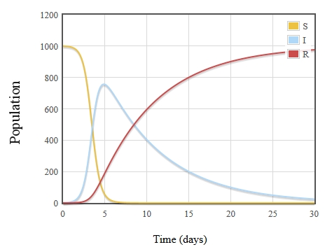
We can now move on to understanding the curve of $i$. It is obvious that $s$ only can decrease from its initial susceptible population as people become infected, and $r$ can only increase, as infected people all eventually recover or die and cannot return to a previous state, but $i$ is of particular interest. This is the curve we are all familiar with seeing on the news. When the talking heads say “flatten the curve”, this is the curve they mean. Let’s first prove that $i$ is in fact the peaked curve we are familiar with seeing. That is, we will prove there exists a time $t_1 \in [0,\infty)$ such that $i$ is increasing on the time interval $[0,t_1)$ and decreasing on $(t_1,\infty)$. We know that $i’=psi-\mu i = (ps-\mu)(i)$, so $i'(t) = (ps-\mu)(i(t))$. Thus, the sign (positive or negative) of $i'(t)$ depends solely on the coefficient term $ps-\mu$. Since $s(t)$ is decreasing, $p(s(t))-\mu$ is decreasing as well. Initially, this term is positive, meaning that $i'(t)$ is positive and thus $i(t)$ is increasing. As time goes on and the coefficient term continues to decrease, however, it will eventually (at a time we will label $t_1$) reach zero (meaning $i'(t)$ has no slope and $i(t)$ stops increasing), and become negative, at which point $i(t)$ begins to decrease. Thus, we have $i(t)$ increasing until its peak at $t_1$, then decreasing thereafter.

We also see that $i(t)$ tends toward $0$ as $t \to \infty$. This makes sense, as the number of susceptible people will decrease as time goes on, so the source dries up, and everyone in state $I$ will eventually go to $R$.

Now, we can finally talk about outbreaks and whether one is occurring or not. The mathematical definition for outbreak is simply when the number of infected individuals is rising, aka when $i'(t)>0$. The outbreak stops, then, at the peak of $i$, at $t_1$.

In the sample graph below, $t_1$ appears to be at day 5, meaning the outbreak is only that portion of time from $t=0 \to t=t_1=5$.

The danger of outbreaks is that the infection rate may rise above the threshold for how many individuals a population can medically treat at once. A simple way we often encode outbreak conditions is with the number $R_0$. This is known as the “basic reproduction number” and is given by $R_0 = \frac{p}{\mu}$. Recall that $p$ is some probability (thus between $0$ and $1$) representing the expected number of infections occurring by an infected individual in unit time and$\frac{1}{\mu}$ is the expected recovery time. Hence $R_0 = p\frac{1}{\mu}$ is a measure taking into account both how infectious a disease is and how long it takes to recover (note that a long recovery time means more time an infected individual has to continue spreading the disease to $p$ people per unit of time). Hence a high $R_0$, resulting from a high $p$, a high $1/\mu$, or both, is a bad thing.

It is worth noting that an outbreak cannot occur if $R_0 < 1$. They only occur when $R_0 \geq 1$ and $s(0) \leq \frac{1}{R_0}$. The proof of this is left to the reader; this article is quite lengthy already.

Lastly, we will touch upon Herd Immunity, and what that really means. As mentioned above, an outbreak cannot occur if the initial proportion of the population that is susceptible to the disease is less than $\frac{1}{R_0}$. Reaching the point where an outbreak can not occur or can no longer continue (at $t_1$) is called reaching herd immunity. The $R_0$ value of Covid-19 is, as of a mid-April, estimated to be between 1.4 and 5.7, though it is likely much closer to the former than the latter.

Let’s, for example, take $R_0 = 3$. To reach herd immunity, we need $s(0) \leq 1/R_0 = 1/3$, so we need $2/3$ of the population to be NOT susceptible (i.e. infected or recovered/dead). There are three ways to do this:

1) let the disease run its course. Eventually there will be so many people that have had the disease that the remaining susceptible people are hard to find, and we’ll achieve herd immunity. This is a bad idea.
2) kill prematurely a massive portion of the susceptible population, thus sending them right to state $R$. This is a worse idea.
3) Evacuate, without killing, as much of the susceptible population as possible from state $S$ to state $R$, aka vaccinations.

As we can see, to prevent an outbreak entirely, it is important to find some way to break the rules of our Markov chain, and establish a way to take individuals in state $S$ and transfer them immediately into state $R$, avoiding infecting everyone in the process.

Let’s say we have again $R_0 = 3$. Say we have $99$% of the population in state $S$ and $1$% are infected. By vaccinating a fraction of the people in $S$, we can make them immune and shove them right into $R$ safe and sound. Let’s say at the beginning stages of this disease outbreak ($r = 0.1$) we vaccinate $60$% of the population, leaving $30$% in $S$. Then $s(0) < 1/3$ so $1/R_0 < 1/3$ and herd immunity is reached, and the outbreak is immediately stifled.

And there we have it, the mathematical basis of the SIR model, along with a few examples at the end to see how some of the concepts lead to ideas we might already be familiar with, like flattening the curve and herd immunity. My parting advice is to always be skeptical; do your own research and think for yourself. Everyone has an agenda, and times of crisis and mass fear are when people are most susceptible to being taken advantage of. Understanding how the systems around you actually work is key. I would also like to note that some of these concepts are drawn from lectures given in my Math 531 (Real Analysis) and Math 340 (Adv. Probability Theory) classes.