Section1: IMU data filtering — Junyan Zhou

· Introduction, Research& Education Problem:

The IMU (Inertial Measurement Unit) serves as the critical ‘inner ear’ for a two-wheeled self-balancing robot. It captures essential data on angular velocity and acceleration to estimate the robot’s tilt angle (pitch).

However, raw sensor signals are  subject to noise and drift. Currently, the mainstream filtering algorithm for balance cars is Complementary Filtering. While this method is intuitive, its reliance on fixed parameters makes it unable to adapt to varying noise or dynamic environmental conditions. 

Theoretically, the balance robot can be regarded as a pendulum with no friction and with instantaneous motor response. However, practical challenges include battery voltage fluctuations, unstable mechanical center of gravity, sensor noise, and electronic component installation issues (e.g., MPU6050 pins not properly soldered on the circuit board, causing significant sway that affects attitude angles). Therefore, his work focuses on making a reliable balance robot model, implementing robust filtering algorithms to fuse the IMU data. Since two-wheeled balance robot and bipedal-wheeled robot are essentially in the class of pendulum model, his work will verify the effectiveness of the more robust filtering algorithm, which is the foundation for the control system to maintain the future bipedal-wheeled robot’s dynamic stability.

· Building Experimental Platform

Step 1: Connectivity test

At the beginning he chose ESP32 as circuit board, MPU6050 as IMU, connected on a breadboard, and tested on PlatformIO in VSCode. The output data is shown in VSCode terminal in Fig 1. This step is to test if IMU is connected to microcontroller.

 

Fig 1 raw data output in VSCode

He wrote a script to visualize Roll-Pitch-Yaw data, so that when the breadboard is tilted in different directions, wave form makes corresponding changes, as shown in Fig 2. Note that data is sent to a webpage by WiFi, so time delay is normal. When the IMU later connect to the circuit board, time delay can be ignored. This step is to test if IMU is working normally, and if the data is reasonable. If so it is expected to be responsive to tilting, and the waveform should exhibit corresponding oscillations, including amplitude, angle class and direction. To further explain this, when the breadboard tilts about y-axis, It is expected to see the curve corresponding to Pitch angle oscillates most heavily, the heavier tilt the breadboard has, the larger the amplitude of the curve should be, counterclockwise and clockwise tilting should relate to two sides of the curve.

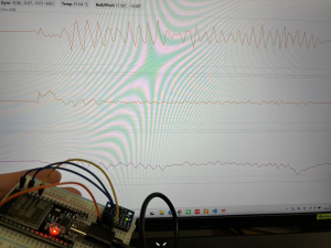
Fig 2 Visualization of RPY angles

Step 2: IMU-motor test

To test if IMU data can be applied onto motor successfully, he wrote a script that control a stepper motor rotating direction using pitch angle, as shown in Fig 3. When the IMU tilts forward, the motor rotates forward; when tilting backward, the motor rotates backward.

Fig 3 IMU data applied on motor test

Step 3: Prototyping

Merely aligning the motor direction with the tilt angle is insufficient. To validate the effectiveness of the filtering algorithms, he prototyped a self-balancing robot. The process is outlined below.

He chose two TT DC motors (with wheels), Elegoo Nano V3 as microcontroller, MPU6050 as IMU,  TB6612FNG as motor driver, a 6v battery pack, and a breadboard, as shown in Fig 4.

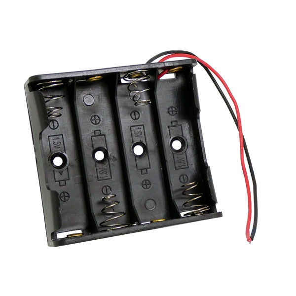
Fig 4 *Pictures are all from Google Images.* (from left to right) TT DC motors (with wheels), Elegoo Nano V3, MPU6050,  TB6612FNG, a 6v battery pack, a breadboard.

The breadboard was adhered to the robot chassis. The only thing that needs to pay attention to is the position of each module. He assembled them together so that its center of mass is in the same plane that goes across two wheels’ centers. It ensures that when placed properly, the robot should be at static balance, which makes dynamic balancing feasible.

The final product is shown in Fig 5.

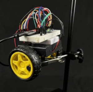
Fig 5 two-wheeled self balancing robot

· Experiment Design

The goal is to compare the performance between no filter, Complementary Filter and Adaptive Complementary Filter. Raw IMU signals are imperfect: accelerometers suffer from high-frequency noise due to vibrations, while gyroscopes accumulate drift over time. Filtering is essential to fuse these signals, combining long-term accelerometer stability with short-term gyroscope precision for an accurate angle estimate. A standard complementary filter uses a fixed gain to merge these signals. In contrast, an adaptive complementary filter dynamically adjusts this gain based on real-time motion conditions, such as total acceleration.

 

From CF to ACF, coefficient alpha switches from a fixed one alpha, to a time-dependent one alpha_k. The advantage of the adaptive approach is improved robustness during dynamic situations. By automatically reducing reliance on the accelerometer when external acceleration is detected, it prevents large angle errors during fast movements while remaining computationally simple.[1]

To verify this , he set three scenarios altogether. Two scenarios are common in a real world robot running case and one static scenarios, which are static, slow motion, forward. The experimental setup is illustrated in Fig 6 and Fig 7.

Fig 6 Robot on a stand

Fig 6 shows the setup for static scenario. The robot is held on a stand so it’s static.

Fig 7 Robot on desk

Fig 7 shows the setup for slow motion and forward scenarios. Notice that two coins are placed on the robot so that when it’s released it will go forward because of the effect of coin mass. The coins are glued and there is a cable connected to his laptop in real tests.

· Videos:

CF:

ACF:

· Data Analysis

For each scenario, he conducted the experiment for unfiltered, CF and ACF, generating 4 figures for each filter case (Pitch, Roll, Gyro, Accelerometer). That would be 3*3*4=36 figures in total. In a robot balancing case, Pitch angle and gyro are the most important to focus since they make more sense in keeping balance. Also to some extent in order to keep the website concise, only Pitch and Gyro figures in each case are selected and put on the website.

1.Static (from left to right, Unfiltered, CF, ACF, applied to all)

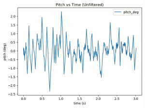
-Pitch

-Gyro

In static pitch experiments, all three filtering methods exhibit varying degrees of drift, with the offset direction trending toward negative values. The unfiltered data near the zero point suggests that data noise dominates the drift effect, making the drift less noticeable. In gyro experiments, unlike the other two groups, the CF’s xyz-axis data showed closer alignment. At system startup, the y-axis rotational angular velocity initially exceeded those of the other two axes, gradually stabilizing near zero. This phenomenon likely stems from the system’s high acceleration during initial operation. CF’s over-correction mechanism may generate excessive torque in the motor, causing the y-axis angular velocity to spike momentarily (also, it could simply be an outlier). The unusually small x-axis value at t=0 is likely an outlier, possibly due to uneven surfaces on the experimental table or other factors that induced a sharp roll angle change.

2.Slow Motion

-Pitch

-Gyro

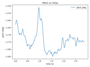
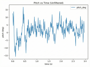
In the pitch angle experiment for slow motion, The introduction of motion makes the data change more violently. Under normal conditions, the unfiltered pitch angle should theoretically have a larger oscillation amplitude than the CF. However, in this experiment, the two values were nearly identical (the unfiltered one was slightly 20% higher), which may be due to the inherent limitations of the MPU6050.

3.Forward

-Pitch

-Gyro

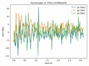
The CF graph from the gyro experiment vividly illustrates the issues caused by CF. When the robot accelerates horizontally, CF’s excessive error correction causes oscillatory overshoots, which is reflected in the graph as the angular velocity on the y-axis fluctuating periodically with a direction that significantly exceeds the values of the other two axes. Generally, the y-axis data shows more obvious changes compared to the other two axes. This is because the robot’s tilting is most noticeable during movement. The second most significant change is the yaw angle on the z-axis, which may result from the robot’s turning due to an uneven table surface.

Overall analysis:

To analyze the performance of unfiltered data, the Complementary Filter (CF), and the Adaptive Complementary Filter (ACF), three metrics are introduced: noise level (jitter), amplitude, and drift. It can be observed that from left to right, amplitude of oscillation decreases.

The unfiltered signal is highly unstable and jagged, which is primarily caused by the high-frequency vibration of the accelerometer and the random walk of the gyroscope. Also the intrinsic properties of MPU6050 is a key factor, since this IMU model is a cost-effective one and may not be ideally stable.

The CF algorithm suppresses this noise by fusing the low-frequency stability of the accelerometer with the high-frequency response of the gyroscope. However, it may still show slight overshoots or lags during rapid motion if the parameters are not optimized.

In contrast, the ACF further optimizes performance by dynamically adjusting the gain based on external acceleration. This method effectively reduces external disturbances, leading to a trajectory that is sharper and more accurate.

· Code for ACF（Run on Arduino IDE)

· Future Work

Although the robot using ACF is significantly more stable than the one using CF, it eventually falls down after a period of slight oscillation. This indicates that while ACF effectively suppresses noise, it cannot withstand continuous external disturbances.

The main reason is that he only applied a Proportional (P) controller to the DC motors. Without derivative action to dampen the overshoot, the robot fails to recover from severe oscillations caused by huge center-of-mass shifts. To achieve continuous self-balancing in the future, PID or PD control is a basic requirement. Several potential approaches can be implemented:

1.Encoder wheel

It consists of a slotted plastic disc (usually 20 or 40 slots) attached to the motor’s output shaft and a photo-interrupter sensor. As the wheel spins, the disc blocks and passes the light beam. The sensor outputs a digital pulse (0 or 1) for each slot passed. For hardware, the sensor on the chassis needs to be mounted on the disc on the wheel, connecting the sensor’s signal pin to an Arduino External interrupt pin. Speed is calculated by:

Pulse Count / Slots per Revolution * Time

This approach is intuitive and low-cost while it cannot tell the direction and its resolution is relatively low. A 20-slot disc means 18° rotation per pulse, which leads to oscillation.

2.Encoder motor

It integrates a magnetic Hall effect sensor and a magnetic disc on the rear shaft of the motor (before the gearbox). As the motor spins, the sensor detects the changing magnetic field and outputs two square wave signals (Phase A and Phase B) with a 90-degree phase shift. The motor has 6 wires (2 for power, 4 for the encoder). Connect Phase A and B to the microcontroller’s interrupt pins.

Total Pulses per Revolution = Encoder PPR * Gear Ratio

It has very high resolution and precise direction, even when the speed is low it provides good feeback, but the drawbacks are relatively high cost and complexity because it has more pins so for hardware and software there’s going to be extra works. With more advanced MCU and encoder motor, we can also try more complex control and filter algorithms, like LQR and Kalman Filter.[2]

· References

[1] Z. Zhang, J. Wang, B. Song, and G. Tong, “Adaptive Complementary Filtering Algorithm for IMU Based on MEMS,” in 2020 Chinese Control and Decision Conference (CCDC), Hefei, China, 2020, pp. 5409–5414, doi: 10.1109/CCDC49329.2020.9164809.

This paper explains that standard complementary filters fail during high-dynamic motion because the accelerometer confuses external vibrations with gravity. It proposes an adaptive algorithm that dynamically reduces reliance on the accelerometer when external acceleration is detected, ensuring accurate and stable attitude estimation.

[2] V. Klemm et al., “Ascento: A Two-Wheeled Jumping Robot,” in 2019 International Conference on Robotics and Automation (ICRA), Montreal, QC, Canada, 2019, pp. 3783–3789, doi: 10.1109/ICRA.2019.8794081.

This paper introduces a  two-wheeled jumping robot that utilizes a parallel linkage mechanism to structurally decouple jumping impact from the balancing dynamics. They propose a control framework combining an LQR algorithm for stabilization and an Extended Kalman Filter (EKF) for state estimation, enabling the robot to perform agile jumping maneuvers while maintaining robust self-balancing.