
For high-dimensional data, dimensionality reduction (DR) methods have been invaluable tools for human understanding, as they can map datasets into two or three dimensions for visualization, providing an intuitive way to understand the data. In recent years, tons of DR methods for data visualization have been proposed, and some are much better than others. In this blog post, we explore several DR methods, discuss how to determine which methods are effective, and explain why some are better than others.
In this blog post, we analyze the following DR methods. We also notice that this is far from a comprehensive list – there exists hundreds of other DR methods being designed for different domains every year.
- t-SNE
- UMAP
- PaCMAP
- PHATE
- LargeVis
- TriMap
- HNNE
- HeatGeo
- Principal Components Analysis (PCA)
There also exist lots of variants of t-SNE/UMAP with slightly different loss functions that behave similarly to t-SNE and UMAP, including NCVis, InfoNC-t-SNE, and Neg-t-SNE. For conciseness, we won’t discuss those variants here.
As a preview of the rest of this blog post, we’ll see that for data visualization, LargeVis, TriMap, PCA, PHATE, HeatGeo and h-NNE fail to pass some basic sanity check testing. We are much better off using the other DR methods. t-SNE, while it is the most well-known, does not consistently handle global structure well. UMAP has less problems with global structure, but PaCMAP is simply better at handling global structure (and we’ll explain why). We’ll also touch on cases where no DR method can perform well, showing the limits of current DR methods.
Just to be clear, we’re talking only about data visualization here. PCA and other methods can still be useful for reducing dimensions as a preprocessing step. But PCA is not useful for data visualization because (as you will see) it does not handle local structure preservation at all.
An important note about performance metrics: There are many performance metrics available for DR, but since it’s unsupervised, it’s not clear whether any of them work particularly well. They are designed to capture whether the 2D visualization is faithful to our knowledge about the structure of the high-dimensional data. In our experience, current quantitative performance metrics generally aren’t that useful if you already know what you’re looking for visually. For instance, if you know there are 3 clusters in the data and you see 3 clusters in the DR plot, that will be more powerful than a number that comes out of a performance metric. What you actually perceive tells you more about the quality of the algorithms in those cases. So in what follows, we’ll show DR results on data where we already know the structure of the data in high dimensions so you can judge these methods for yourself without dealing with questionable performance metrics.
The MNIST Test
The classic MNIST data is a dataset of 70,000 handwritten digits of the shape 28 x 28. Due to its simplicity, it has been widely used as a basic benchmark for machine learning and DR algorithms. The MNIST dataset can effectively verify the ability of the DR algorithm to preserve the local structure. If the method doesn’t work on MNIST, it’s generally considered inadequate.
The MNIST test evaluates the local structure preservation ability of the DR method, which is the preservation of neighborhoods. Specifically, points that are close in the original high dimensional space should also be close in low dimensional space. We know that MNIST consists of images from 10 separated digits and has 10 separated clusters in high-dimensions pixel space. As a result, a trustworthy DR method should also map the dataset into 10 separated clusters in low-dimensions. If the DR method can’t separate the data into clusters of digits, then it doesn’t pass the test.
Below are the data visualizations of MNIST generated by all the methods. We gave some methods the benefit of the doubt by including multiple parameter settings, but as we’ll discuss below, this approach isn’t really fair, as the user doesn’t know in advance which parameters to choose due to DR’s unsupervised nature.
Figure 1. MNIST dataset, projected to 2 dimensions using several different DR methods. Note that HeatGeo is not supported for large datasets (>20,000 samples) within limited memory, so we sampled 2,000 points of each label for DR visualization. MNIST actually has 10 clusters that are separated in high dimensions. Algorithms that don’t pass this sanity check include PCA, LargeVis (which created more than 10 clusters), PHATE, hNNE and HeatGeo. Algorithms that passed (including methods that blurred some clusters) include t-SNE, UMAP, PaCMAP, and TriMAP.
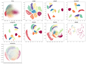
Figure 1. MNIST dataset, projected to 2 dimensions using several different DR methods. Note that HeatGeo is not supported for large datasets (>20,000 samples) within limited memory, so we sampled 2,000 points of each label for DR visualization. MNIST actually has 10 clusters that are separated in high dimensions. Algorithms that don’t pass this sanity check include PCA, LargeVis (which created more than 10 clusters), PHATE, hNNE and HeatGeo. Algorithms that passed (including methods that blurred some clusters) include t-SNE, UMAP, PaCMAP, and TriMAP.
The Mammoth Test
The Mammoth dataset is a 3D dataset of points on a mammoth. The task is to project to 2D while preserving the general shape of the mammoth.
The mammoth test evaluates the global structure preservation ability of DR methods. Global structure is the preservation of clusters and manifolds, or larger scale structures. If cluster A is farther than cluster B from cluster C, their relationship should be reflected in the DR projection. If a cluster exists in high dimensions that is split into two clusters in low dimensions, global structure is not preserved.
Below are DR plots of all the methods on the mammoth data. If global structure is preserved, the mammoth should still visibly look like a mammoth. But for many of these DR methods, it doesn’t. Here, PCA can get it right since the two principal components are the length and height of the mammoth.

Figure 2: Mammoth dataset, projected onto 2D using different DR methods. Methods that didn’t pass the sanity check include t-SNE, UMAP, LargeVis, PHATE, HNNE, and HeatGeo. Algorithms that passed are PCA, PaCMAP, and TriMap.
We’ll repeat this experiment on a couple more datasets where global structure is important. The COIL20 dataset is next, which consists of 20 high-dimensional coils (i.e., rings). Clearly some of these algorithms are better than others. Our usual suspects (UMAP, PaCMAP, TriMap) do pretty well, whereas the others do not. Similar results follow on the COIL100 dataset, which has 100 high-dimensional coils.

Figure 3a: COIL20 Dataset, projected onto 2D using different DR methods. Methods that didn’t pass the sanity check include PCA, t-SNE, LargeVis, PHATE, HNNE, and HeatGeo, though one could argue that even though LargeVis and t-SNE broke apart some of the coils, their results at least show that the data live on a curve. Algorithms that passed are UMAP, PaCMAP, and TriMap.

Figure 3b. COIL100 Dataset projected onto 2D using different DR methods. Similar results as in Figure 3a.
The next dataset is the “synthetic hierarchical” dataset. This dataset is particularly difficult for DR methods. It consists of 5 “macro clusters” that each have 5 “meso clusters,” and each of the meso subclusters has 5 “micro clusters.” Thus, there are 5x5x5 = 125 micro clusters total. We colored each point based on its true macro clusters, shading each meso cluster. The DR plot should convey this. However, many of the DR methods don’t get it right. UMAP’s DR plot mixes up the positions of all the meso clusters so you can’t see the clusters at all. The other usual high-performers (t-SNE, PaCMAP, TriMap) perform well along with PCA, though TriMap seems to be a cut above the rest here.
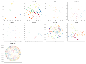
Figure 4. Synthetic Hierarchical Dataset with 125 clusters (125 micro clusters within 25 meso cluster and within 5 macro clusters) projected onto 2D using different DR methods
Next is the S-curve-with-a-hole dataset. Like the Mammoth, this is a 3D object projected onto 2D. Only TriMap and PaCMAP perform well, displaying the S-curve and the hole in it.
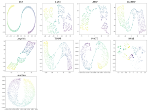
Figure 5. S Curve with a hole projected onto 2D using different DR methods
The results so far from LargeVis, HNNE, HeatGeo and PHATE, have been pretty bad. Let us go into more detail on t-SNE, UMAP, and PaCMAP, whose results are generally better, even if UMAP and t-SNE aren’t able to handle global structure very well.
Robustness to Parameter Adjustment
t-SNE and UMAP are sensitive to parameters, as we’ll see in the images below. PaCMAP is not so sensitive due to how it’s optimized. Let’s explain this a bit more by considering the forces of t-SNE and UMAP (this is taken from https://jmlr.org/papers/v22/20-1061.html). Both of them have attractive forces and repulsive forces, but those forces alone do not shape global structure. In the following plot below on the left is the 2D curve dataset. A DR method should have just left the points where it was, but in the figure on the right, it did not. (On the right is the DR result of UMAP.)

Figure 6. Left: 2D curve dataset. Right: UMAP’s result. Points that were supposed to be close to each other are close (nearest neighbors) and points that were supposed to be far from each other are far, but global structure is not preserved.
Think about a loss function for the DR projection whose goal is to keep neighbors close and keep non-neighbors far. The UMAP result in the figure minimizes this loss perfectly – all the neighbors are close and the further points are far. But its global structure is totally wrong!
The key to preserving global structure used by PaCMAP is to exert attractive forces much further than just the local neighborhood, so that the global structure is shaped by these much longer scale attractive forces.
Since t-SNE and UMAP don’t optimize global structure, they basically get it from PCA initialization. If you remove the PCA initialization, their results get much worse! PaCMAP’s global forces prevent this from happening and make its results much more robust.

Figure 7. PCA initialization makes a big difference for t-SNE, UMAP, and TriMAP, but not PaCMAP, whose solutions are more robust.
Now that this is explained, let’s now show the robustness results in experiments. For t-SNE, the mammoth looks better (but never really good) when we tune the parameter very high. However, the high parameters aren’t the optimal parameter settings for MNIST. This means that no matter what parameter setting we choose for t-SNE, it will be bad for either one or both types of datasets. Again these are unsupervised methods, so you normally don’t know how to tune the parameters – mammoth and MNIST (and the other datasets considered here) are unusual because we actually know the ground truth. Ideally, the parameters should be fixed so no one needs to try to tune them.

Figure 8. t-SNE, UMAP, and TriMap with various parameter settings. PaCMAP has no parameters that are designed to be tuned.

Figure 9: t-SNE, LargeVis, UMAP, and TriMap with various parameter settings. PaCMAP has no parameters that are designed to be tuned.
Robustness to initialization
Since DR is unsupervised, if the DR method provides different results with different initialization or on different runs, users don’t know which one of these plots to trust. Figure 8 shows that most methods, with the exception of PaCMAP, aren’t able to produce consistent DR embeddings. The most concerning observations are that TriMap is doing very poorly on MNIST most of the time, UMAP breaks the data up into more than 10 clusters, and t-SNE also seems to have problems with parts of clusters breaking off – these types of results could be really misleading to biologists looking for distinct cell types for instance.
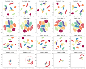
Figure 10: Different initial conditions on MNIST.
We hope you enjoyed this blog post that sheds light on the performance of the DR algorithms! We’ll try to post updates to it as more competitive DR methods become available. Obviously we don’t want to update every time someone creates a new variant of t-SNE since there are thousands of those, but we’ll try to update when there’s really different new approaches that become available.
— Haiyang Huang, Yingfan Wang, Yiyang Sun, Gaurav Parikh, Cynthia Rudin — July 5, 2024