Category: Algorithms

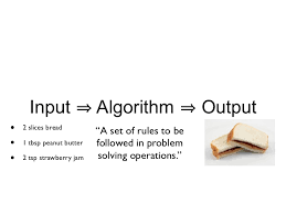
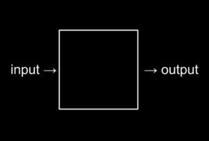
In Computer Science, we are often challenged to “do better” ― even though our program works, we are asked to make it run faster or use up less space. Since there are often different ways to implement a solution to the same problem, different algorithms that achieve the same goal can yield wide-ranging time and space complexities. Why might the running time of an algorithm matter? Simply put, an algorithm is ultimately useless if it takes forever to run ― we never get our desired output. Why might the space that an algorithm takes up matter? Space can be expensive sometimes. However, as memory is becoming cheaper and cheaper with advancements in technology, programmers are usually willing to trade more space for a faster runtime. Let me illustrate the tradeoffs between time and space complexity by analyzing two different ways of solving the Fibonacci problem. 

The Fibonacci Problem:

The Fibonacci Sequence is a famous series of numbers shown below:

0, 1, 1, 2, 3, 5, 8, 13, 21, 34, 55, 89, 144, 233, 377, 610, 987, 1597, 2584

As you can see, the first number is 0, the second number is 1, and the next numbers are the sum of the two numbers before it:

• The 2 is found by adding the two numbers before it (1+1),
• The 3 is found by adding 1+2,
• The 5 is found by adding 2+3,
• And so on… 

When we try to picture the Fibonacci Sequence using squares, we see a nice spiral! 5 and 8 make 13, 8 and 13 make 21, and so on… 

Turns out this spiral property of Fibonacci sequences are also seen prevalently in real life, especially in nature. 

We are now tasked to solve the Fibonacci problem: Given any positive integer n, find the nth number in the Fibonacci Sequence. We could, of course, calculate this by hand. If we want to find the 5th Fibonacci number, we could just start from the first two Fibonacci numbers and follow the definition until we get to the 5th term: 0, 1, 1 (0+1), 2 (1+1), 3 (1+2). However, this start-from-scratch method quickly becomes impractical as n gets large ― it would be a huge waste of time for us to manually calculate the 1000th Fibonacci number! Thus, we turn to a computer to help us solve this problem. 

Naive Recursive Solution: 

Using Python (or another programming language), we can implement a simple recursive program that computes the nth Fibonacci number.

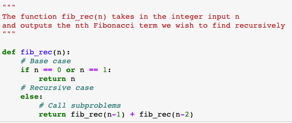
For an input of 5 to our naive recursive solution, we can observe the pattern above. In a tree-like structure, fib5 (fib_rec(5)) is broken down into fib4 and fib3, fib4 is broken down into fib3 and fib2, fib3 is broken down into fib2 and fib1, and finally fib2 is broken down to our base cases: fib1 and fib0, which evaluate to 1 and 0 respectively. The recursive algorithm then uses our known base case values to compute all the other subproblems (e.g. fib2, fib3, etc…) in a bottom up approach. It is important to note that without our base cases specified, our algorithm would not work because there would be no stopping point. In this case, a stack overflow error would be thrown. 

Scanning the diagram from top to bottom, we notice that as we move downwards, each layer of fib items grows exponentially in size. Layer 0 has 1 (2^0) item,  layer 1 has 2 (2^1) items, layer 2 has 4 (2^2) items, layer 3 has the potential for 8 (2^3) items, layer 4 has the potential for 16 (2^4) items, and layer n has the potential for 2^n items. Since adding more inputs means adding more fib layers with items growing exponentially, the time complexity of our solution is O(2^n). This turns out to be very inefficient for even not-so-large input sizes like 50 or 100. For example, while fib_rec(40) takes a few seconds to run, fib_rec(80) takes theoretically years to run. While it is still feasible to solve small Fibonacci numbers with our naive recursive solution, we cannot solve large Fibonacci numbers using this approach. 

Dynamic Programming Solution:

Can we do better? 

When brainstorming for more optimal solutions, we can begin by analyzing the flaws of our less optimal solution. In the recursive tree diagram, we notice that there are a lot of overlapping computations. For instance, fib2 is repeatedly calculated 3 times and fib3 is repeatedly calculated 2 times. While this may not seem like a lot, the exponential increase of overlapping computations will add up when we have larger inputs, such as 50 or 100. What if we store the results of these repeated computations somewhere? Then, we can use them directly instead of recomputing when we need them. This “memoized” (memo = a note recording something for future use) solution is a common problem-solving strategy known as Dynamic Programming (DP). 

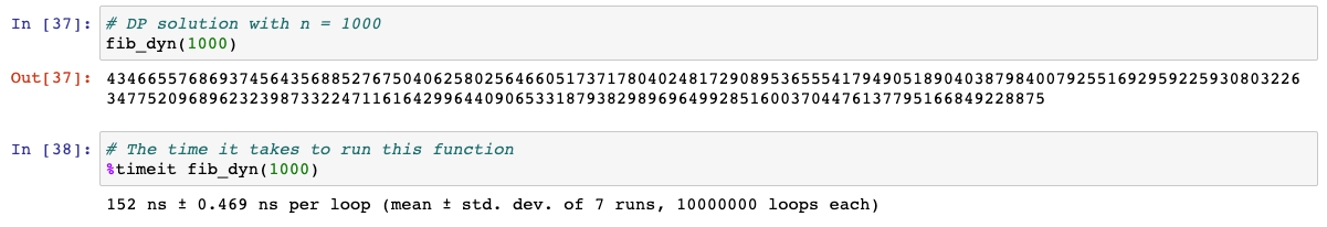
Before we define the function fib_dyn(n), we first create an array with null (empty) values that acts as a cache, or a structure that stores data so that future requests for that data can be served faster. Trading space for speed, we store the value of fib0 at index 0 of the cache array, fib1 at index 1, fib2 at index 2, etc… To compute a new fib value, we just need to look up the previous two entries in the cache array. With our base cases defined, we can simply use cache[0] and cache[1] to find cache[2], cache[1] and cache[2] to find cache[3], etc…, successfully avoiding the unnecessary overlapping computations. The time complexity for our DP solution is O(n) (linear) for traversing the cache array, which is significantly faster than our O(2^n) (exponential) recursive solution. The only downside of our DP solution is the added space complexity of O(n) for creating the cache array. This downside, however, is minuscule compared to the amazing benefit of a drastically reduced time complexity. In fact, I was able to run fib_dyn(1000) and get the accurate result almost instantly.

Conclusion:

Here are several key takeaways from this post:

1. Programmers care about how fast a program runs and how much space it takes up because these attributes dramatically impact user experience. 
2. When looking for a more optimal solution, examine the flaws of the less optimal solution and identify patterns. Find a way to get around the flaws (with perhaps a new data structure), and develop your improved solution from there. 
3. Trading space for speed is encouraged in most situations. 

They are everywhere. 

From social media apps and search engines to video streaming sites and dating apps, algorithms are everywhere in our modern, technology-driven world. 

But what exactly is an algorithm? 

How do they work? 

Who makes them? 

And should we be worried about them? 

Let’s figure out. 

Definition

With a quick Google search, we see that an algorithm is defined as “a process or set of rules to be followed in calculations or other problem-solving operations, especially by a computer.” This might sound like a riddle to you. There are so many definitions on the internet that do not clearly explain what algorithms actually do. I’m here to help!

A non-internet based example of an algorithm is a cookbook recipe. A recipe provides a set of instructions to specify how you should put together several ingredients to get a product (eg. sandwich) on the other end. In the peanut butter and jelly sandwich example above, we are given 2 slices of bread, 1 tablespoon of peanut butter, and 2 tablespoons of strawberry jam as inputs to our algorithm. The algorithm we use to make the sandwich might include the following procedures: 

1. Gather Your Ingredients for the Sandwich
2. Pull Out Two Slices of Bread
3. Open Peanut Butter and Jelly
4. Spread the Peanut Butter Onto One Slice of Bread
5. Spread the Jelly Onto the Other Slice of Bread
6. Combine the Two Slices

After completing the instructions specified by the algorithm, we are able to accurately produce our output  ― a delicious peanut butter and jelly sandwich! 

Algorithms in Computer Science

An algorithm in Computer Science does effectively the same thing ― it is a set of instructions that enables a computer program to put together different input sources and output a result. 

While a programmer implements code to specify the algorithm for recommending new YouTube videos or which post you see first on your Facebook feed, users are usually unaware of how an algorithm is designed. As a user, you can treat an algorithm as a “black box” – you provide valid input information and wait to see the magic happen. When we use Google Maps to find the fastest route to a destination, we don’t need to worry about what computations we need to make to locate the shortest path (thank god!). We simply provide the algorithm with relevant input information such as our starting point, destination, and mode of travel and the algorithm automatically generates the best path for us. This principle of removing unnecessary details (e.g. how the shortest path is computed) to boost user experience is a recurring concept in Computer Science known as “abstraction”. 

Correctness

How do we know if an algorithm is well-designed? We can start with analyzing its “correctness”. It is likely that you have experienced the frustrations of dealing with a poorly-designed algorithm yourself. When I was child, my parents purchased a new car GPS navigator. On a road trip, the GPS incorrectly led us to a rural farm and instructed us to drive into a field of crops. Luckily, we quickly disregarded the misguided directions and eventually found our way back on track. In this case, the GPS algorithm was “incorrect”. In other words, it failed to produce the correct output we were looking for ― a feasible path to our final destination. In certain high-stakes situations, incorrect algorithms can even yield life-or-death consequences. On March 19, 2018, an Uber self-driving car running in autonomous mode hit and killed a woman walking on a poorly lit road. According to Uber, the algorithm incorrectly classified the women as “unknown object”, then “vehicle”, and then “bicycle” during the brief encounter. It is this indecisiveness that led to a very late action (stopping the car), which eventually caused the tragedy. Algorithms are useful when they are correct, helping us automate tedious tasks, find valuable information, and perform complex procedures. On the other hand, incorrect algorithms do more harm than good, from wasting time to even taking lives. 

Efficiency

We can also analyze an algorithm by evaluating its “efficiency”. Going back to the Google Map example: What if a search for the fastest route to a nearby destination takes an hour? If driving to the destination only takes 15 minutes on average, there is no point in making the search before traveling there. Even if we choose a slower route from our memory, we would still arrive at the destination faster than waiting for the app recommendation result and taking the fastest route. This shows how even if an algorithm is correct, it is ultimately unhelpful if it takes too much time to run. 

Conclusion

Algorithms are not as difficult to understand as many people think ― they show up in many facets of our daily lives and help us better utilize the resources around us.