Home » Articles posted by Jonathan Mattingly
Author Archives: Jonathan Mattingly
Girsanov Example
Let \(u(x)\colon \mathbf{R}^d \rightarrow \mathbf{R}^d\) such that \(\sup_x |u(x)| \leq K \). Define \(X_t\) by
\[dX_t = u(X_t)dt + \sigma dB_t\]
for \(\sigma >0\) and \(X_0=x\).
For any open set \( A \subset \mathbf{R}^d\) assume that you know that \(P(B_t \in A) >0)\) show that the same holds for \(X_t\).
Hint: Start by showing that \(\mathbf{E}[ f(x+ \sigma B_t)] = \mathbf{E}[\Lambda_t f(X_t)]\) for some process \(\Lambda_t\) and any function \(f\colon \mathbf{R}^d\rightarrow \mathbf{R}\). Next show that \(\mathbf{E}[\Lambda_t^2] < \infty\)
Exit Through Boundary II
Consider the following one dimensional SDE.
\begin{align*}
dX_t&= \mu dt+ \sin( X_t )^\alpha dW(t)\\
X_0&=\frac{\pi}2
\end{align*}
Consider the equation for \(\alpha >0\) and \(\mu \in \mathbf{R}\). On what interval do you expect to find the solution at all times ? Classify the behavior at the boundaries in terms of the parameters.
For what values of \(\alpha < 0\) does it seem reasonable to define the process ? any ? justify your answer.
Practice with Ito Formula
Let \(B_t\) be a standard Brownian motion. For each of the following definitions of \(Y_t\), find adapted stochastic process \(\mu_t\) and \(\sigma_t\) so that \(dY_t =\mu_t dt + \sigma_t dB_t\)
- \( Y_t =\sin(B_t) \)
- \( Y_t= (B_t)^p \) for \(p>0\)
- \( Y_t=\exp( B_t – t^2)\)
- \(Y_t=\log(B_t) \)
- \(Y_t= t^2 B_t \)
Product Chain
Let \(Z_n\) be a collection of independent random variables with \(P(Z_n=1)=\frac12\) and \(P(Z_n=\frac12)=\frac12\) . Define \(X_0=1\) and \(X_{n+1}=Z_n X_n\).
- What is \(E( X_n | X_{n-1})\) ?
- What is \(E(X_n)\) ?
- What is \(\mathrm{Cov}(X_n,X_{n-1})\) ?
Basic Markov Chain I
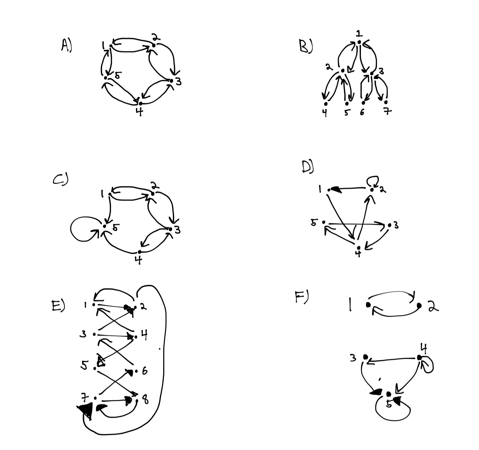
In each of the graphs pictured, assume that each arrow leaving a vertex has an equal chance of being followed. Hence if there are thee arrows leaving a vertex then there is a 1/3 chance of each being followed.
- For each of the six pictures, find the Markov transition matrix.
- State if the Markov chain given by this matrix is irreducible.
- If the Matrix is irreducible, state if it is aperiodic.
Conditional Variance
Given two random variables, we define the conditional variance of \(X\) given \(Y\) by
\[ \text{Var}(X | Y ) = E(X^2 | Y ) – (\,E(X | Y )\,)^2 \]
Show that
\[ \text{Var}(X ) = E (\text{Var}(X | Y ) ) +\text{Var}( E(X | Y ) ) \,. \]
Of course \( E(X | Y )\) is just random variable so we have that
\[ \text{Var}( E(X | Y ) ) = E [\,E(X | Y )^2\,] – [\,E(\,E(X | Y )\,)\,]^2 \]
also is is useful to recall that \(E(E(X | Y ))= E(X )\).
Random Walk
Let \(\{Z_1, Z_2, \dots, Z_n,\dots\} \) be a sequence of i.i.d random variables such that
\[ P( Z_k = a ) = \begin{cases} \frac14 & \text{ If } a=1 \\\frac14 & \text{ If } a=0\\\frac12 & \text{ If } a=-1 \end{cases}\]
If \(X_{n+1} = X_n + Z_n\) and \(X_0=1\) what is
- \( E( X_{n+1} | X_{n}) \)?
- \( E( X_{n+1}) \)?
- \( \text{Var}( X_{n+1} | X_{n}) \)?
- \( \text{Var}( X_{n+1} )\)?
Notice that \(X_n\) depends only \(Z_{n-1},Z_{n-2},\dots,Z_1\) and hence \(X_n\) is independent of \(Z_n\) !
Joint Density Poisson arrival
Let \(T_1\) and \(T_5\) be the times of the first and fifth arrivals in a Poisson arrival prices with rate \(\lambda\). Find the joint distribution of \(T_1\) and \(T_5\) .
Uniform Spacing
Let \(U_1, U_2, U_3, U_4, U_5\) be independent uniform \((0,1)\) random variables. Let \(R\) be the difference between the max and the min of the random variables. Find
- \( E( R)\)
- the joint density of the min and the max of the \(U\)’s
- \(P( R>0.5)\)
[Pitman p. 355 #14]
Joint density part 2
Let \(X\) and \(Y\) have joint density
\(f(x,y) = 90(y-x)^8, \quad 0<x<y<1\)
- State the conditional distribution of \(X \mid Y\) and \(Y \mid X\)
- Are these two random variables independent?
- What is \( \mathbf{P}(Y \mid X=.2 ) \) and \( \mathbf{E}(Y \mid X=.2) \) ?
What is \( \mathbf{P}(Y \mid X=.2 ) \) and \( \mathbf{E}(Y \mid X=.2) \)
[Adapted from Pitman pg 354]
Uniform distributed points given an arrival
Consider a Poisson arrival process with rate \(\lambda>0\). Let \(T\) be the time of the first arrival starting from time \(t>0\). Let \(N(s,t]\) be the number of arrivals in the time interval \((s,t]\).
Fixing an \(L>0\), define the pdf \(f(t)\) by \(f(t)dt= P(T \in dt | N(0,L]=1)\) for \(t \in (0,L]\). Show that \(f(t)\) is the pdf of a uniform random variable on the interval \([0,L]\) (independent of \(\lambda\) !).
Cognitive Dissonance Among Monkeys
Assume that each monkey has a strong preference between red, green, and blue M&M’s. Further, assume that the possible orderings of the preferences are equally distributed in the population. That is to say that each of the 6 possible orderings ( R>G>B or R>B>G or B>R>G or B>G>R or G>B>R or G>R>B) are found with equal frequency in the population. Lastly assume that when presented with two M&Ms of different colors they always eat the M&M with the color they prefer.
In an experiment, a random monkey is chosen from the population and presented with a Red and a Green M&M. In the first round, the monkey eats the one based on their personal preference between the colors. The remaining M&M is left on the table and a Blue M&M is added so that there are again two M&M’s on the table. In the second round, the monkey again chooses to eat one of the M&M’s based on their color preference.
- What is the chance that the red M&M is not eaten in the first round?
- What is the chance that the green M&M is not eaten in the first round?
- What is the chance that the Blue M&M is not eaten in the second round?
[Mattingly 2022]
Which deck is rigged ?
Two decks of cards are sitting on a table. One deck is a standard deck of 52 cards. The other deck (called the rigged deck) also has 52 cards but has had 4 of the 13 Harts replaced by Diamonds. (Recall that a standard deck has 4 suits: Diamonds, Harts, Spades, and Clubs. normal there are 13 of each suit.)
- What is the probability one chooses 4 cards from the rigged deck and gets exactly 2 diamonds and no hearts?
- What is the probability one chooses 4 cards from the standard deck and gets exactly 2 diamonds and no hearts?
- You randomly chose one of the decks and draw 4 cards. You obtain exactly 2 diamonds and no hearts.
- What is the probability you chose the cards from the rigged deck?
- What is the probability you chose the cards from the standard deck?
- If you had to guess which deck was used, which would you guess? The standard or the rigged ?
Getting your feet wet numerically
Simulate the following stochastic differential equations:
- \[ dX(t) = – \lambda X(t) dt + dW(t) \]
- \[ dY(t) = – \lambda Y(t) dt +Y(t) dW(t) \]
by using the following Euler type numerical approximation
- \[X_{n+1} = X_n – \lambda X_n h + \sqrt{h} \eta_n\]
- \[Y_{n+1} = Y_n – \lambda Y_n h + \sqrt{h} Y_n\eta_n\]
where \(n=0,1,2,\dots\) and \(h >0\) is a small number that give the numerical step side. That is to say that we consider \( X_n \) as an approximation of \(X( t) \) and \( Y_n \) as an approximation of \(Y( t) \) each with \(t=h n\). Here \(\eta_n\) are a collection of mutually independent random variables each with a Gaussian distribution with mean zero and variance one. (That is \( N(0,1) \).)
Write code to simulate the two equations using the numerically methods suggested. Plot some trajectories. Describe how the behavior changes for different choices of \(\lambda\). Can you conjecture where it changes ? Compare and contrast the behavior of the two equations.
Tell your story with pictures.
Handing back tests
A professor randomly hands back test in a class of \(n\) people paying no attention to the names on the paper. Let \(N\) denote the number of people who got the right test. Let \(D\) denote the pairs of people who got each others tests. Let \(T\) denote the number of groups of three who none got the right test but yet among the three of them that have each others tests. Find:
- \(\mathbf{E} (N)\)
- \(\mathbf{E} (D)\)
- \(\mathbf{E} (T)\)
Up by two
Suppose two teams play a series of games, each producing a winner and a loser, until one time has won two more games than the other. Let \(G\) be the number of games played until this happens. Assuming your favorite team wins each game with probability \(p\), independently of the results of all previous games, find:
- \(P(G=n) \) for \(n=2,3,\dots\)
- \(\mathbf{E}(G)\)
- \(\mathrm{Var}(G)\)
[Pittman p220, #18]
Population
A population contains \(X_n\) individuals at time \(n=0,1,2,\dots\) . Suppose that \(X_0\) is distributed as \(\mathrm{Poisson}(\mu)\). Between time \(n\) and \(n+1\) each of the \(X_n\) individuals dies with probability \(p\) independent of the others. The population at time \(n+1\) is comprised of the survivors together with a random number of new immigrants who arrive independently in numbers distributed according to \(\mathrm{Poisson}(\mu)\).
- What is the distribution of \(X_n\) ?
- What happens to this distribution as \(n \rightarrow \infty\) ? Your answer should depended on \(p\) and \(\mu\). In particular, what is \( \mathbf{E} X_n\) as \(n \rightarrow \infty\) ?
[Pittman [236, #18]
A modified Wright-Fisher Model
Consider the ODE
\[ \dot x_t = x_t(1-x_t)\]
and the SDE
\[dX_t = X_t(1-X_t) dt + \sqrt{X_t(1-X_t)} dW_t\]
- Argue that \(x_t\) can not leave the interval \([0,1]\) if \( x_0 \in (0,1)\).
- What is the behavior of \(x_t\) as \(t \rightarrow\infty\) if if \( x _0\in (0,1)\) ?
- Can the diffusion \(X_t\) exit the interval \( (0,1) \) ? Prove your claims.
- What do you think happens to \(X_t\) as \(t \rightarrow \infty\) ? Argue as best you can to support your claim.
No Explosions from Diffusion
Consider the following ODE and SDE:
\[\dot x_t = x^2_t \qquad x_0 >0\]
\[d X_t = X^2_t dt + \sigma |X_t|^\alpha dW_t\qquad X_0 >0\]
where \(\alpha >0\) and \(\sigma >0\).
- Show that \(x_t\) blows up in finite time.
- Find the values of \(\sigma\) and \(\alpha\) so that \(X_t\) does not explode (off to infinity).
[ From Klebaner, ex 6.12]
Cox–Ingersoll–Ross model
The following model has SDE has been suggested as a model for interest rates:
\[ dr_t = a(b-r_t)dt + \sigma \sqrt{r_t} dW_t\]
for \(r_t \in \mathbf R\), \(r_0 >0\) and constants \(a\),\(b\), and \(\sigma\).
- Find a closed form expression for \(\mathbf E( r_t)\).
- Find a closed form expression for \(\mathrm{Var}(r_t)\).
- Characterize the values of parameters of \(a\), \(b\), and \(\sigma\) such that \(r=0\) is an absorbing point.
- What is the nature of the boundary at \(0\) for other values of the parameter ?
SDE Example: quadratic geometric BM
Show that the solution \(X_t\) of
\[ dX_t=X_t^2 dt + X_t dB_t\]
where \(X_0=1\) and \(B_t\) is a standard Brownian motion has the representation
\[ X_t = \exp\Big( \int_0^t X_s ds -\frac12 t + B_t\Big)\]
Practice with Ito and Integration by parts
Define
\[ X_t =X_0 + \int_0^t B_s dB_s\]
where \(B_t\) is a standard Brownian Motion. Show that \(X_t\) can also be written
\[ X_t=X_0 + \frac12 (B^2_t -t)\]
Discovering the Bessel Process
Let \(W_t=(W^{(1)}_t,\dots,W^{(n)}_t) \) be an \(n\)-dimensional Brownian motion with \( W^{(i)}_t\) standard independent 1-dim brownian motions and \(n \geq 2\).
Let
\[X_t = \|W_t\| = \Big(\sum_{i=1}^n (W^{(i)}_t)^2\Big)^{\frac12}\]
be the norm of the brownian motions. Even though the absolute value is not differentiable at zero we can still apply Itos formula since Brownian motion never visits the origin if the dimension is greater than zeros.
- Use Ito’s formula to show that \(X_t\) satisfies the Ito process
\[ dX_t = \frac{n-1}{2 X_t} dt + \sum_{i=1}^n \frac{W^{(i)}_t }{X_t} dW^{(i)}_t \] - Using the Levy-Doob Theorem show that
\[Z_t =\sum_{i=1}^n \int_0^t \frac{W^{(i)}_t }{X_t} dW^{(i)}_t \]
is a standard Brownian Motion. - In light of the above discussion argue that \(X_t\) and \(Y_t\) have the same distribution if \(Y_t\) is defined by
\[ dY_t = \frac{n-1}{2 Y_t} dt + dB_t\]
where \(B_t\) is a standard Brownian Motion.
Take a moment to reflect on what has been shown. \(W_t\) is a \(\mathbf R^n\) dimensional Markov Process. However, there is no guarantee that the one dimensional process \(X_t\) will again be a Markov process, much less a diffusion. The above calculation shows that the distribution of \(X_{t+h}\) is determined completely by \(X_t\) . In particular, it solves a one dimensional SDE. We were sure that \(X_t\) would be an Ito process but we had no guarantee that it could be written as a single closed SDE. (Namely that the coefficients would be only functions of \(X_t\) and not of the details of the \(W^{(i)}_t\)’s.
One dimensional stationary measure
Consider the one dimensional SDE
\[dX_t = f(X_t) dt + g(X_t) dW_t\]
which we assume has a unique global in time solution. For simplicity let us assume that there is a positive constant \(c\) so that \( 1/c < g(x)<c\) for all \(x\) and that \(f\) and \(g\) are smooth.
A stationary measure for the problem is a probability measure \(\mu\) so that if the initial distribution \(X_0\) is distributed according to \(\mu\) and independent of the Brownian Motion \(W\) then \(X_t\) will be distributed as \(\mu\) for any \(t \geq 0\).
If the functions \(f\) and \(g\) are “nice” then the distribution at time \(t\) has a density with respect to Lebesgue measure (“dx”). Which is to say there is a function \(p_x(t,y)\) do that for any \(\phi\)
\[\mathbf E_x \phi(X_t) = \int_{-\infty}^\infty p_x(t,y)\phi(y) dy\]
and \(p_\phi(t,y)\) solves the following equation
\[\frac{\partial p_\phi}{\partial t}(t,y) = (L^* p_\phi)(t,y)\]
with \( p_\phi(0,y) = \phi(y)\) where \(\phi(z)\) is the density with respect to Lebesgue of the initial density. (The pdf of \(X_0\) .)
\(L^*\) is the formal adjoint of the generator \(L\) of \(X_t\) and is defined by
\[(L^*\phi)(y) = – \frac{\partial\ }{\partial y}( f \phi)(y) + \frac12 \frac{\partial^2\ }{\partial y^2}( g^2 \phi)(y) \]
Since we want \(p_x(t,y)\) not to change when it is evolved forward with the above equation we want \( \frac{\partial p}{\partial t}=0\) or in other words
\[(L^* p_\phi)(t,y) =0\]
- Let \(F\) be such that \(-F’ = f/g^2\). Show that \[ \rho(y)=\frac{K}{g^2(y)}\exp\Big( – 2F(y) \Big)\] is an invariant density where \(K\) is a normalization constant which ensures that
\[\int \rho(y) dy =1\] - Find the stationary measure for each of the following SDEs:
\[dX_t = (X_t – X^3_t) dt + \sqrt{2} dW_t\]\[dX_t = – F'(X_t) dt + \sqrt{2} dW_t\] - Assuming that the formula derived above make sense more generally, compare the invariant measure of
\[ dX_t = -X_t + dW_t\]
and
\[ dX_t = -sign(X_t) dt + \frac{1}{\sqrt{|X_t|}} dW_t\] - Again, proceding fromally assuming everything is well defined and makes sense find the stationary density of \[dX_t = – 2\frac{sign(X_t)}{|X_t|} dt + \sqrt{2} dW_t\]
Numerical SDEs – Euler–Maruyama method
If we wanted to simulate the SDE
\[dX_t = b(X_t) dt + \sigma(X_t) dW_t\]
on a computer then we truly want to approximate the associated integral equation over a sort time time interval of length \(h\). Namely,
\[X_{t+h} – X_t= \int_t^{t+h}b(X_s) ds + \int_t^{t+h}\sigma(X_s) dW_s\]
It is reasonable for \(s \in [t,t+h]\) to use the approximation
\begin{align}b(X_s) \approx b(X_t) \qquad\text{and}\qquad\sigma(X_s)\approx \sigma(X_t)\end{align}
which implies
\[X_{t+h} – X_t\approx b(X_t) h + \sigma(X_t) \big( W_{t+h}-W_{t}\big)\]
Since \(W_{t+h}-W_{t}\) is a Gaussian random variable with mean zero and variance \(h\), this discussion suggests the following numerical scheme:
\[ X_{n+1} = X_n + b(X_n) h + \sigma(X_n) \sqrt{h} \eta_n\]
where \(h\) is the time step and the \(\{ \eta_n : n=0,\dots\}\) are a collection of mutually independent standard Gaussian random variable (i.e. mean zero and variance 1). This is called the Euler–Maruyama method.
Use this method to numerically approximate (and plot) several trajectories of the following SDEs numerically.
- \[dX_t = -X_t dt + dW_t\]
- For \(r=-1, 0, 1/4, 1/2, 1\)
\[ dX_t = r X_t dt + X_t dW_t\]Does it head to infinity or approach zero ?Look at different small \(h\). Does the solution go negative ? Should it ? - \[dX_t = X dt -X_t^3 dt + \alpha dW_t\]
Try different values of \(\alpha\). For example, \(\alpha = 1/10, 1, 2 ,10\). How does it act ? What is the long time behavior ? How does it compare with what is learned in the “One dimensional stationary measure” problem about the stationary measure of this equation.
BDG Inequality
Consider \(I(t)\) defined by \[I(t)=\int_0^t \sigma(s,\omega)dB(s,\omega)\] where \(\sigma\) is adapted and \(|\sigma(t,\omega)| \leq K\) for all \(t\) with probability one. Inspired by problem “Homogeneous Martingales and Hermite Polynomials” Let us set
\begin{align*}Y(t,\omega)=I(t)^4 – 6 I(t)^2\langle I \rangle(t) + 3 \langle I \rangle(t)^2 \ .\end{align*}
- Quote the problem “Ito Moments” to show that \(\mathbb{E}\{ |Y(t)|^2\} < \infty\) for all \(t\). Then verify that \(Y_t\) is a martingale.
- Show that \[\mathbb{E}\{ I(t)^4 \} \leq 6 \mathbb{E} \big\{ \{I(t)^2\langle I \rangle(t) \big\}\]
- Recall the Cauchy-Schwartz inequality. In our language it states that
\begin{align*}
\mathbb{E} \{AB\} \leq (\mathbb{E}\{A^2\})^{1/2} (\mathbb{E}\{B^2\})^{1/2}
\end{align*}
Combine this with the previous inequality to show that\begin{align*}\mathbb{E}\{ I(t)^4 \} \leq 36 \mathbb{E} \big\{\langle I \rangle(t)^2 \big\} \end{align*} - We know that \(I^4\) is a submartingale (because \(x \mapsto x^4\) is convex). Use the Kolmogorov-Doob inequality and all that we have just derived to show that
\begin{align*}
\mathbb{P}\left\{ \sup_{0\leq s \leq T}|I(s)|^4 \geq \lambda \right\} \leq ( \text{const}) \frac{ \mathbb{E}\left( \int_0^T \sigma(s,\omega)^2 ds\right)^2 }{\lambda}
\end{align*}
Homogeneous Martingales and Hermite Polynomials
- Let \(f(x,y):\mathbb{R}^2 \rightarrow \mathbb{R}\) be a twice differentiable function in both \(x\) and \(y\). Let \(M(t)\) be defined by \[M(t)=\int_0^t \sigma(s,\omega) dB(s,\omega)\]. Assume that \(\sigma(t,\omega)\) is adapted and that \(\mathbf{E} M^2 < \infty\) for all \(t\) a.s. .(Here \(B(t)\) is standard Brownian Motion.) Let \([M]_t\) be the quadratic variation process of \(M(t)\). What equation does \(f\) have to satisfy so that \(Y(t)=f(M(t),[M]_t)\) is again a martingale if we assume that \(\mathbf E\int_0^t \sigma(s,\omega)^2 ds < \infty\).
- Set
\begin{align*}
f_n(x,y) = \sum_{0 \leq m \leq \lfloor n/2 \rfloor} C_{n,m} x^{n-2m}y^m
\end{align*}
here \(\lfloor n/2 \rfloor\) is the largest integer less than or equal to \(n/2\). Set \(C_{n,0}=1\) for all \(n\). Then find a recurrence relation for \(C_{n,m+1}\) in terms of \(C_{n,m}\), so that \(Y(t)=f_n(B(t),t)\) will be a martingale.Write out explicitly \(f_1(B(t),t), \cdots, f_4(B(t),t)\) as defined in the previous item. - Again let \(M(t)=\int_0^t \sigma(s,\omega) dB(s,\omega)\) with \(|\sigma(t,\omega)| < K\) almost surely. Show that \(f_n(M(t),[M]_t)\) is again a martingale where \([M]_t\) is the quadratic variation of \(M(t)\) and \(f_n\) is the function found above.
- * Do you recognize the recursion relation you obtained above for \(f_n\) as being associated to a famous recursion relation ? (Hint: Look at the title of the problem)
Using the Cauchy–Schwarz inequality
Recall that the Cauchy–Schwarz inequality stats that for any two random variable \(X\) and \(Y\) one has that
\[ \mathbf E |XY| \leq \sqrt{\mathbf E [X^2]}\,\sqrt{ \mathbf E [Y^2]}\]
- Use it to show that
\[ \mathbf E |X| \leq \sqrt{\mathbf E [X^2]}\]
Ito Variation of Constants
For functions \(f(x)\) and\( g(x) \) and constant \(\beta>0\), define \(X_t\) as the solution to the following SDE
\[dX_t = – \beta X_t dt + h(X_t)dt + g(X_t) dW_t\]
where \(W_t\) is a standard Brownian Motion.
- Show that \(X_t\) can be written as
\[X_t = e^{-\beta t} X_0 + \int_0^{t} e^{-\beta (t-s)} h(X_s) ds + \int_0^{t} e^{-\beta (t-s)} g(X_s) dW_s\]
See exercise: Ornstein–Uhlenbeck process for guidance. - Assuming that \(|h(x)| < K\) and \(|g(x)|<K\), show that there exists a constant \(C(X_0)\) so that
\[ \mathbf E [|X_t|] < C(X_0) \]
for all \(t >0\). It might be convenient the remember the Cauchy–Schwarz inequality. - * Assuming that \(|h(x)| < K\) and \(|g(x)|<K\), show that for any integer \(p >0\) there exists a constant \(C(p,X_0)\) so that
\[ \mathbf E [|X_t|^{2p}] < C(p,X_0) \]
for all \(t >0\). See exercise: Ito Moments for guidance.
Ornstein–Uhlenbeck process
For \(\alpha \in \mathbf R\) and \(\beta >0\), Define \(X_t\) as the solution to the following SDE
\[dX_t = – \beta X_t dt + \alpha dW_t\]
where \(W_t\) is a standard Brownian Motion.
- Find \( d(e^{\beta t} X_t)\) using Ito’s Formula.
- Use the calculation of \( d(e^{\beta t} X_t)\) to show that
\begin{align} X_t = e^{-\beta t} X_0 + \alpha \int_0^t e^{-\beta(t-s)} dW_s\end{align} - Conclude that \(X_t\) is Gaussian process (see exercise: Gaussian Ito Integrals ). Find its mean and variance at time \(t\).
- * Let \(h(t)\) and \(g(t)\) be deterministic functions of time and let \(Y_t\) solve
\[dY_t = – \beta Y_t dt + h(t)dt+ \alpha g(t) dW_t\]
show find a formula analogous to part 2 above for \(Y_t\) and conclude that \(Y_t\) is still Gaussian. Find it mean and Variance.
Exponential Martingale
Let \(\sigma(t,\omega)\) be adapted to the filtration generated by a standard Brownian Motion \(B_t\) such that \(|\sigma(x,\omega)| < K\) for some bound \(K\) . Let \(I(t,\omega)=\int_0^t \sigma(s,\omega) dB(s,\omega)\).
- Show that
\[M_t=\exp\big\{\alpha I(t)-\frac{\alpha^2}{2}\int_0^t \sigma^2(s)ds \big\}\]
is a martingale. It is called the exponential martingale. - Show that \(M_t\) satisfies the equation
\[ dM_t =\alpha M_t dI_t = \alpha M_t \sigma_t dB_t\]
Ito Integration by parts
Recall that if \(u(t)\) and \(v(t)\) are deterministic functions which are once differentiable then the classic integration by parts formula states that
\[ \int_0^t u(s) (\frac{dv}{ds})(s)\,ds = u(t)v(t) – u(0)v(0) – \int_0^t v(s) (\frac{du}{ds})(s)\,ds\]
As is suggested by the formal relations
\[ (\frac{dv}{ds})(s)\,ds=dv(s) \qquad\text{and}\qquad (\frac{du}{ds})(s)\, ds=du(s)\]
this can be rearranged to state
\[ u(t)v(t)- u(0)v(0)= \int_0^t u(s) dv(s) + \int_0^t v(s) du(s)\]
which holds for more general Riemann–Stieltjes integrals. Now consider two Ito processes \(X_t\) and \(Y_t\) given by
\[dX_t=b_s ds + \sigma_s dW_t \qquad\text{and}\qquad dY_t=f_s ds + g_s dW_t \]
where \(W_t\) is a standard Brownian Motion. Derive the “Integration by Parts formula” for Ito calculus by applying Ito’s formula to \(X_tY_t\). Compare this the the classical formula given above.
Cross-quadratic variation: correlated Brownian Motions
Let \(W_t\) and \(B_t\) be two independent standard Brownian Motions. For \(\rho \in [0,1]\) define
\[ Z_t = {\rho}\, W_t +\sqrt{1-\rho^2}\, B_t\]
- Why is \(Z_t\) a standard Brownian Motion ?
- Calculate the cross-quadratic variations \([ Z,W]_t\) and \([ Z,B]_t\) .
- For what values of \(\rho\) is \(W_t\) independent of \(Z_t\) ?
- ** Argue that two standard Brownian motions are independent if and only if their cross-quadratic variation is zero.
Paley-Wiener-Zygmund Integral
Definition of stochastic integrals by integration by parts
In 1959, Paley, Wiener, and Zygmund gave a definition of the stochastic integral based on integration by parts. The resulting integral will agree with the Ito integral when both are defined. However the Ito integral will have a much large domain of definition. We will now follow the develop the integral as outlined by Paley, Wiener, and Zygmund:
- Let \(f(t)\) be a deterministic function with \(f'(t)\) continuous. Prove that \begin{align*} \int_0^1 f(t)dW(t) = f(1)W(1) – \int_0^1 f'(t)W(t) dt\end{align*}
where the first integral is the Ito integral and the last integral is defined path-wise as the standard Riemann integral since the integrands are a.s. continuous. - Now let \(f\) we as above with in addition \(f(1)=0\) and “define” the stochastic integral \(\int_0^1 f(t) * dW(t)\) by the relationship
\begin{align*}
\int_0^1 f(t) *dW(t) = – \int_0^1 f'(t) W(t) dt\;.
\end{align*}
Where the integral on the right hand side is the standard Riemann integral.If the condition \(f(1)=0\) seems unnatural to you, what this is really saying is that \(f\) is supported on \([0,1)\). In many ways it would be most natural to consider \(f\) on \([0,\infty)\) with compact support. Then \(f(\infty)=0\). We consider the unit interval for simplicity.
- Show by direct calculation (not by the Ito isometry) that
\begin{align*}
\mathbf E \left[ \left(\int_0^1 f(t)* dW(t)\right)^2\right]=\int_0^1 f^2(t) dt\;,
\end{align*}
Paley, Wiener, and Zygmund then used this isometry to extend the integral to any deterministic function in \(L^2[0,1]\). This can be done since for any \(f \in L^2[0,1]\), one can find a sequence of deterministic functions in \(\phi_n \in C^1[0,1]\) with \(\phi_n(1)=0\) so that
\begin{equation*}
\int_0^1 (f(s) – \phi_n(s))^2ds \rightarrow 0 \text{ as } n \rightarrow 0\,.
\end{equation*}
Stratonovich integral: A first example
Let us denote the Stratonovich integral of a standard Brownian motion \(W(t)\) with respect to itself by
\begin{align*}
\int_0^t W(s)\circ dW(t)\;.
\end{align*}
we then define the integral buy
\begin{align*}
\int_0^t W(s)\circ dW(t) = \lim_{n \rightarrow \infty}
\sum_k\frac12\big(W(t_{k+1}^n)+W(t_{k}^n)\big)\big(W(t_{k+1}^n) -W(t_{k}^n)\big)
\end{align*}
where \(t_k^n=k\frac{t}n\). Prove that with probability one
\begin{align*}
X_t= \int_0^t W(s)\circ dW(s)= \frac12 W(t)^2\;.
\end{align*}
Observe that this is what one would have if one used standard (as opposed to Ito) calculus. Calculate \(\mathbf E [ X_t | \mathcal{F}_s]\) for \(s < t\) where \(\mathcal{F}_t\) is the \(\sigma\)-algebra generated by the Brownian motion. Is \(X_t\) a martingale with respect to \(\mathcal{F}_t\).